Using Vectors
Numerical Precision and Topology Exceptions
When doing any significant amount of geometric computation, there is the potential of encountering JTS TopologyExceptions or other numerical hiccups that arise, essentially, from asking too much of floating point numerical representations. JTS offers the ability to snap coordinates to a grid, the scale of whose cells may be specified by the user. This can often fix problems stemming from numerical error which makes two points that should be the same appear different due to miniscule rounding errors.
However, GeoTrellis defaults to allowing the full floating point
representation of coordinates. To enable the fixed precision scheme, one must
create an application.conf in your-project/src/main/resources/
containing the following lines:
geotrellis.jts.precision.type="fixed"
geotrellis.jts.precision.scale=<scale factor>
The scale factor should be 10^x where x is the number of decimal
places of precision you wish to keep. The default scale factor is 1e12,
indicating that 12 decimal places after the decimal point should be kept.
Values less than 1 (negative exponents) allow for very coarse grids. For
example, a scale factor of 1e-2 will round coordinate components to the
nearest hundred.
Note that geotrellis.jts.precision.type make take on the value
floating for the default double precision case, or floating_single to
use single precision floating point values.
These parameters will be reflected in the system geometry factory available in geotrellis.vector.GeomFactory.factory.
Parsing GeoJson
GeoTrellis includes good support for serializing and deserializing
geometry to/from GeoJson within the geotrellis.vector.io.json
package. Utilizing these features requires some instruction, however,
since the interface may not be immediately apparent from the type
signatures.
Serializing to GeoJson
All Geometry and Feature objects in geotrellis.vector have a
method extension providing a toGeoJson method. This means that:
import geotrellis.vector.io._

Polygon((10.0, 10.0), (10.0, 20.0), (30.0, 30.0), (10.0, 10.0)).toGeoJson
is valid, in this case yielding:
{"type":"Polygon","coordinates":[[[10.0,10.0],[10.0,20.0],[30.0,30.0],[10.0,10.0]]]}
Issuing .toGeoJson on Feature instances, requires that the type
parameter supplied to the feature meets certain requirements. For
example, PointFeature(Point(0,0), 3) will succeed, but to tag a
Feature with arbitrary data, that data must be encapsulated in a case
class. That class must also be registered with the Json reading
infrastructure provided by spray. The following example achieves
these goals:
import geotrellis.vector.io.json._

case class UserData(data: Int)
implicit val boxedValue = jsonFormat1(UserData)

PointFeature(Point(0,0), UserData(13))
Case classes with more than one argument would require the variants of
jsonFormat1 for classes of higher arity. The output of the above
snippet is:
{"type":"Feature","geometry":{"type":"Point","coordinates":[0.0,0.0]},"properties":{"data":13}}
where the property has a single field named data. Upon
deserialization, it will be necessary for the data member of the feature
to have fields with names that are compatible with the members of the
feature’s data type.
This is all necessary underpinning, but note that it is generally
desirable to (de)serialize collections of features. The serialization
can be achieved by calling .toGeoJson on a Seq[Feature[G, T]].
The result is a Json representation of a FeatureCollection.
Deserializing from GeoJson
The return trip from a string representation can be accomplished by
another method extension provided for strings: parseGeoJson[T]. The
only requirement for using this method is that the type of T must
match the contents of the Json string. If the Json string represents
some Geometry subclass (i.e., Point, MultiPolygon, etc),
then that type should be supplied to parseGeoJson. This will work to
make the return trip from any of the Json strings produced above.
Again, it is generally more interesting to consider Json strings that
contain FeatureCollection structures. These require more complex
code. Consider the following Json string:
val fc: String = """{
                   |  "type": "FeatureCollection",
                   |  "features": [
                   |    {
                   |      "type": "Feature",
                   |      "geometry": { "type": "Point", "coordinates": [1.0, 2.0] },
                   |      "properties": { "someProp": 14 },
                   |      "id": "target_12a53e"
                   |    }, {
                   |      "type": "Feature",
                   |      "geometry": { "type": "Point", "coordinates": [2.0, 7.0] },
                   |      "properties": { "someProp": 5 },
                   |      "id": "target_32a63e"
                   |    }
                   |  ]
                   |}""".stripMargin
Decoding this structure will require the use of either
JsonFeatureCollection or JsonFeatureCollectionMap; the former
will return queries as a Seq[Feature[G, T]], while the latter will
return a Map[String, Feature[G, T]] where the key is the id
field of each feature. After calling:
val collection = fc.parseGeoJson[JsonFeatureCollectionMap]
it will be necessary to extract the desired features from
collection. In order to maintain type safety, these results are
pulled using accessors such as .getAllPoints,
.getAllMultiLineFeatures, and so on. Each geometry and feature type
requires the use of a different method call.
As in the case of serialization, to extract the feature data from this
example string, we must create a case class with an integer member named
someProp and register it using jsonFormat1.
case class SomeProp(someProp: Int)
implicit val boxedToRead = jsonFormat1(SomeProp)

collection.getAllPointFeatures[SomeProp]
A Note on Creating JsonFeatureCollectionMaps
It is straightforward to create FeatureCollection representations, as
illustrated above. Simply package your features into a Seq and call
toGeoJson. In order to name those features, however, it requires
that a JsonFeatureCollectionMap be explicitly created. For instance:
val fcMap = JsonFeatureCollectionMap(Seq("bob" -> Feature(Point(0,0), UserData(13))))
Unfortunately, the toGeoJson method is not extended to
JsonFeatureCollectionMap, so we are forced to call
fcMap.toJson.toString to get the same functionality. The return of
that call is:
{
  "type": "FeatureCollection",
  "features": [{
    "type": "Feature",
    "geometry": {
      "type": "Point",
      "coordinates": [0.0, 0.0]
    },
    "properties": {
      "data": 13
    },
    "id": "bob"
  }]
}
Working with Vectors in Spark
While GeoTrellis is focused on working with raster data in spark, we do have some functionality for working with vector data in spark.
ClipToGrid
If you have an RDD[Geometry] or RDD[Feature[Geometry, D]], you may want to
cut up the geometries according to SpatialKey s, so that you can join
that data to other raster or vector sources in an efficient way. To do this,
you can use the rdd.clipToGrid methods.
For example, if you want to read GeoTiffs on S3, and find the sum of raster values under each of the polygons, you could use the following technique:
import geotrellis.raster._
import geotrellis.spark._
import geotrellis.spark.tiling._
import geotrellis.vector._

import org.apache.spark.HashPartitioner
import org.apache.spark.rdd.RDD

import java.net.URI
import java.util.UUID

// The extends of the GeoTiffs, along with the URIs
val geoTiffUris: RDD[Feature[Polygon, URI]] = ???
val polygons: RDD[Feature[Polygon, UUID]] = ???

// Choosing the appropriately resolute layout for the data is here considered a client concern.
val layout: LayoutDefinition = ???

// Abbreviation for the code to read the window of the GeoTiff off of S3
def read(uri: URI, window: Extent): Raster[Tile] = ???

val groupedPolys: RDD[(SpatialKey, Iterable[MultiPolygonFeature[UUID]])] =
  polygons
    .clipToGrid(layout)
    .flatMap { case (key, feature) =>
      val mpFeature: Option[MultiPolygonFeature[UUID]] =
        feature.geom match {
          case p: Polygon => Some(feature.mapGeom(_ => MultiPolygon(p)))
          case mp: MultiPolygon => Some(feature.mapGeom(_ => mp))
          case _ => None
        }
      mpFeature.map { mp => (key, mp) }
    }
    .groupByKey(new HashPartitioner(1000))

val rastersToKeys: RDD[(SpatialKey, URI)] =
  geoTiffUris
    .clipToGrid(layout)
    .flatMap { case (key, feature) =>
      // Filter out any non-polygonal intersections.
      // Also, we will do the window read from the SpatialKey extent, so throw out polygon.
      feature.geom match {
        case p: Polygon => Some((key, feature.data))
        case mp: MultiPolygon => Some((key, feature.data))
        case _ => None
      }
    }

val joined: RDD[(SpatialKey, (Iterable[MultiPolygonFeature[UUID]], URI))] =
  groupedPolys
    .join(rastersToKeys)

val totals: Map[UUID, Long] =
  joined
    .flatMap { case (key, (features, uri)) =>
      val raster = read(uri, layout.mapTransform.keyToExtent(key))

      features.map { case Feature(mp, uuid) =>
        (uuid, raster.tile.polygonalSum(raster.extent, mp).toLong)
      }
    }
    .reduceByKey(_ + _)
    .collect
    .toMap
Kriging Interpolation
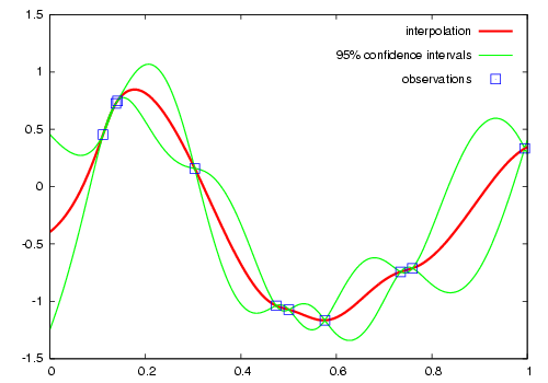
Semivariograms
This method of interpolation is based on constructing Semivariograms. For grasping the structure of spatial dependencies of the known data-points, semivariograms are constructed.
First, the sample data-points’ spatial structure to be captured is converted to an empirical semivariogram, which is then fit to explicit/theoretical semivariogram models.
Two types of Semivariograms are developed :
- Linear Semivariogram
- Non-Linear Semivariograms
Empirical Semivariogram
//(The array of sample points)
val points: Array[PointFeature[Double]] = ???

/** The empirical semivariogram generation
  * "maxDistanceBandwidth" denotes the maximum inter-point distance relationship
  * that one wants to capture in the empirical semivariogram.
  */
val es: EmpiricalVariogram = EmpiricalVariogram.nonlinear(points, maxDistanceBandwidth, binMaxCount)
The sample-data point used for training the Kriging Models are clustered into groups(aka bins) and the data-values associated with each of the data-points are aggregated into the bin’s value. There are various ways of constructing the bins, i.e. equal bin-size(same number of points in each of the bins); or equal lag-size(the bins are separated from each other by a certain fixed separation, and the samples with the inter-points separation fall into the corresponding bins).
In case, there are outlier points in the sample data, the equal bin-size approach assures that the points’ influence is tamed down; however in the second approach, the outliers would have to be associated with weights (which is computationally more intensive).
The final structure of the empirical variogram has an array of tuples :
(h, k)
where h => Inter-point distance separation
      k => The variogram's data-value (used for covariogram construction)
Once the empirical semivariograms have been evaluated, these are fitted into the theoretical semivariogram models (the fitting is carried out into those models which best resemble the empirical semivariogram’s curve generate).
Linear Semivariogram
/** "radius" denotes the maximum inter-point distance to be
  * captured into the semivariogram
  * "lag" denotes the inter-bin distance
  */
val points: Array[PointFeature[Double]] = ...
val linearSV = LinearSemivariogram(points, radius, lag)
This is the simplest of all types of explicit semivariogram models and does not very accurately capture the spatial structure, since the data is rarely linearly changing. This consists of the points’ being modelled using simple regression into a straight line. The linear semivariogram has linear dependency on the free variable (inter-point distance) and is represented by:
f(x) = slope * x + intercept
Non-Linear Semivariogram
/**
  * ModelType can be any of the models from
  * "Gaussian", "Circular", "Spherical", "Exponential" and "Wave"
  */
val points: Array[PointFeature[Double]] = ...
val nonLinearSV: Semivariogram =
    NonLinearSemivariogram(points, 30000, 0, [[ModelType]])
Most often the empirical variograms can not be adequately represented by the use of linear variograms. The non-linear variograms are then used to model the empirical semivariograms for use in Kriging intepolations. These have non-linear dependencies on the free variable (inter-point distance).
In case the empirical semivariogram has been previously constructed, it can be fitted into the semivariogram models by :
val svSpherical: Semivariogram =
    Semivariogram.fit(empiricalSemivariogram, Spherical)
The popular types of Non-Linear Semivariograms are :
(h in each of the function definition denotes the inter-point distances)
Gaussian Semivariogram
// For explicit/theoretical Gaussian Semivariogram
val gaussianSV: Semivariogram =
    NonLinearSemivariogram(range, sill, nugget, Gaussian)
The formulation of the Gaussian model is :
                    | 0                                 , h = 0
gamma(h; r, s, a) = |
                    | a + (s - a) {1 - e^(-h^2 / r^2)}  , h > 0
Circular Semivariogram
//For explicit/theoretical Circular Semivariogram
val circularSV: Semivariogram =
    NonLinearSemivariogram(range, sill, nugget, Circular)
                    | 0                                                                        , h = 0
                    |
                    |               |                                              _________ |
                    |               |      2                | h |      2h         /    h^2   |
gamme(h; r, s, a) = | a + (s - a) * |1 - ----- * cos_inverse|---| + -------- *   /1 - -----  | , 0 < h <= r
                    |               |      pi               | r |    pi * r    \/      r^2   |
                    |               |                                                        |
                    |
                    | s                                                                        , h > r
Spherical Semivariogram
// For explicit/theoretical Spherical Semivariogram
val sphericalSV: Semivariogram = NonLinearSemivariogram(range, sill, nugget, Spherical)
                    | 0                             , h = 0
                    |             | 3h      h^3   |
gamma(h; r, s, a) = | a + (s - a) |---- - ------- | , 0 < h <= r
                    |             | 2r     2r^3   |
                    | s                             , h > r
Exponential Semivariogram
// For explicit/theoretical Exponential Semivariogram
val exponentialSV: Semivariogram = NonLinearSemivariogram(range, sill, nugget, Exponential)
                    | 0                                  , h = 0
gamma(h; r, s, a) = |
                    | a + (s - a) {1 - e^(-3 * h / r)}   , h > 0
Wave Semivariogram
//For explicit/theoretical Exponential Semivariogram
//For wave, range (viz. r) = wave (viz. w)
val waveSV: Semivariogram =
    NonLinearSemivariogram(range, sill, nugget, Wave)
                    | 0                                 , h = 0
                    |
gamma(h; w, s, a) = |             |       sin(h / w)  |
                    | a + (s - a) |1 - w ------------ | , h > 0
                    |             |           h       |
Notes on Semivariogram fitting
The empirical semivariogram tuples generated are fitted into the semivariogram models using Levenberg Marquardt Optimization. This internally uses jacobian (differential) functions corresponding to each of the individual models for finding the optimum range, sill and nugget values of the fitted semivariogram.
// For the Spherical model
val model: ModelType = Spherical
valueFunc(r: Double, s: Double, a: Double): (Double) => Double =
    NonLinearSemivariogram.explicitModel(r, s, a, model)
The Levenberg Optimizer uses this to reach to the global minima much faster as compared to unguided optimization.
In case, the initial fitting of the empirical semivariogram generates a negative nugget value, then the process is re-run after forcing the nugget value to go to zero (since mathematically, a negative nugget value is absurd).
Kriging Methods
Once the semivariograms have been constructed using the known point’s values, the kriging methods can be invoked.
The methods are largely classified into different types in the way the mean(mu) and the covariance values of the object are dealt with.
//Array of sample points with given data
val points: Array[PointFeature[Double]] = ...

//Array of points to be kriged
val location: Array[Point] = ...
There exist four major kinds of Kriging interpolation techniques, namely :
Simple Kriging
//Simple kriging, tuples of (prediction, variance) per prediction point
val sv: Semivariogram = NonLinearSemivariogram(points, 30000, 0, Spherical)

val krigingVal: Array[(Double, Double)] =
    new SimpleKriging(points, 5000, sv)
      .predict(location)
/**
  * The user can also do Simple Kriging using :
  * new SimpleKriging(points).predict(location)
  * new SimpleKriging(points, bandwidth).predict(location)
  * new SimpleKriging(points, sv).predict(location)
  * new SimpleKriging(points, bandwidth, sv).predict(location)
  */
It belongs to the class of Simple Spatial Prediction Models.
The simple kriging is based on the assumption that the underlying stochastic process is entirely known and the spatial trend is constant, viz. the mean and covariance values of the entire interpolation set is constant (using solely the sample points)
mu(s) = mu              known; s belongs to R
cov[eps(s), eps(s')]    known; s, s' belongs to R
Ordinary Kriging
//Ordinary kriging, tuples of (prediction, variance) per prediction point
val sv: Semivariogram = NonLinearSemivariogram(points, 30000, 0, Spherical)

val krigingVal: Array[(Double, Double)] =
    new OrdinaryKriging(points, 5000, sv)
      .predict(location)
/**
  * The user can also do Ordinary Kriging using :
  * new OrdinaryKriging(points).predict(location)
  * new OrdinaryKriging(points, bandwidth).predict(location)
  * new OrdinaryKriging(points, sv).predict(location)
  * new OrdinaryKriging(points, bandwidth, sv).predict(location)
  */
It belongs to the class of Simple Spatial Prediction Models.
This method differs from the Simple Kriging appraoch in that, the constant mean is assumed to be unknown and is estimated within the model.
mu(s) = mu              unknown; s belongs to R
cov[eps(s), eps(s')]    known; s, s' belongs to R
Universal Kriging
//Universal kriging, tuples of (prediction, variance) per prediction point

val attrFunc: (Double, Double) => Array[Double] = {
  (x, y) => Array(x, y, x * x, x * y, y * y)
}

val krigingVal: Array[(Double, Double)] =
    new UniversalKriging(points, attrFunc, 50, Spherical)
      .predict(location)
/**
  * The user can also do Universal Kriging using :
  * new UniversalKriging(points).predict(location)
  * new UniversalKriging(points, bandwidth).predict(location)
  * new UniversalKriging(points, model).predict(location)
  * new UniversalKriging(points, bandwidth, model).predict(location)
  * new UniversalKriging(points, attrFunc).predict(location)
  * new UniversalKriging(points, attrFunc, bandwidth).predict(location)
  * new UniversalKriging(points, attrFunc, model).predict(location)
  * new UniversalKriging(points, attrFunc, bandwidth, model).predict(location)
  */
It belongs to the class of General Spatial Prediction Models.
This model allows for explicit variation in the trend function (mean function) constructed as a linear function of spatial attributes; with the covariance values assumed to be known.
For example if :
x(s) = [1, s1, s2, s1 * s1, s2 * s2, s1 * s2]'
mu(s) = beta0 + beta1*s1 + beta2*s2 + beta3*s1*s1 + beta4*s2*s2 + beta5*s1*s2
Here, the “linear” refers to the linearity in parameters (beta).
mu(s) = x(s)' * beta,   beta unknown; s belongs to R
cov[eps(s), eps(s')]    known; s, s' belongs to R
The attrFunc function is the attribute function, which is used for
evaluating non-constant spatial trend structures. Unlike the Simple and
Ordinary Kriging models which rely only on the residual values for
evaluating the spatial structures, the General Spatial Models may be
modelled by the user based on the data (viz. evaluating the beta
variable to be used for interpolation).
In case the user does not specify an attribute function, by default the function used is a quadratic trend function for Point(s1, s2) :
mu(s) = beta0 + beta1*s1 + beta2*s2 + beta3*s1*s1 + beta4*s2*s2 + beta5*s1*s2
General example of a trend function is :
mu(s) = beta0 + Sigma[ beta_j * (s1^n_j) * (s2^m_j) ]
An elaborate example for understanding the attrFunc is mentioned in
the readme file in geotrellis.raster.interpolation along with
detailed illustrations.
Geostatistical Kriging
//Geostatistical kriging, tuples of (prediction, variance) per prediction point
val attrFunc: (Double, Double) => Array[Double] = {
  (x, y) => Array(x, y, x * x, x * y, y * y)
}

val krigingVal: Array[(Double, Double)] =
    new GeoKriging(points, attrFunc, 50, Spherical)
      .predict(location)
/**
  * Geostatistical Kriging can also be done using:
  * new GeoKriging(points).predict(location)
  * new GeoKriging(points, bandwidth).predict(location)
  * new GeoKriging(points, model).predict(location)
  * new GeoKriging(points, bandwidth, model).predict(location)
  * new GeoKriging(points, attrFunc).predict(location)
  * new GeoKriging(points, attrFunc, bandwidth).predict(location)
  * new GeoKriging(points, attrFunc, model).predict(location)
  * new GeoKriging(points, attrFunc, bandwidth, model).predict(location)
  */
It belongs to the class of General Spatial Prediction Models.
This model relaxes the assumption that the covariance is known. Thus, the beta values and covariances are simultaneously evaluated and is computationally more intensive.
mu(s) = x(s)' * beta,   beta unknown; s belongs to R
cov[eps(s), eps(s')]    unknown; s, s' belongs to R
Delaunay Triangulations, Voronoi Diagrams, and Euclidean Distance
When working with vector data, it is often necessary to establish sensible interconnections among a collection of discrete points in ℝ² (the Euclidean plane). This operation supports nearest neighbor operations, linear interpolation among irregularly sampled data, and Euclidean distance, to name only a few applications.
For this reason, GeoTrellis provides a means to compute the Delaunay
triangulation of a set of points. Letting 𝒫 be the input set of points, the
Delaunay triangulation is a partitioning of the convex hull of 𝒫 into
triangular regions (a partition that completely covers the convex hull with no
overlaps). Each triangle, T, has a unique circle passing through all of
its vertices that we call the circumscribing circle of T. The defining
property of a Delaunay triangulation is that each T has a circumscribing
circle that contains no points of 𝒫 in their interiors (note that the vertices
of T are on the boundary of the circumscribing circle, not in the
interior).

Among the most important properties of a Delaunay triangulation is its
relationship to the Voronoi diagram. The Voronoi diagram is another
partitioning of ℝ² based on the points in 𝒫. This time, the partitioning is
composed of convex polygonal regions—one for each point in 𝒫—that completely
cover the plane (some of the convex regions are half open, which is to say
that they may extend to infinity in certain directions). The Delaunay
triangulation of 𝒫 is the dual to the Voronoi diagram of 𝒫. This means that
elements of the Delaunay triangulation have a one-to-one correspondence with
the elements of the Voronoi diagram. Letting DT(𝒫) be the Delaunay
triangulation of 𝒫 and V(𝒫) be the Voronoi diagram of 𝒫, we have that each
vertex 𝓅 of DT(𝒫) corresponds to a polygonal region of V(𝒫) (called
the Voronoi cell of 𝓅), each edge to an edge, and each triangle to a vertex.
The number of edges emanating from a vertex in DT(𝒫) gives the number of
sides of the corresponding polygonal region in V(𝒫). The corresponding
edges of each structure are perpendicular. The Voronoi vertex corresponding to
a triangle of DT(𝒫) is the center of that triangle’s circumscribing
circle. And if there are no more than 3 points of 𝒫 lying on any circle in
the plane (a condition called general position), then there are no more than
3 edges emanating from any vertex of V(𝒫), which matches the number of
sides in each planar region of DT(𝒫). (If we are not in general
position, not all vertices of V(𝒫) will be distinct and some Voronoi edges
may have zero length.)
The dual relationship between DT(𝒫) and V(𝒫) is important because it
means that we may compute whichever structure that is easiest and simply
derive the other in a straightforward manner. As it happens, it is generally
easier to compute Delaunay triangulations, and we have implemented a very fast
method for doing just that. Specifically, we employ the divide-and-conquer
approach to computing the Delaunay triangulation based on Guibas and Stolfi’s
1985 ACM Transactions on Graphics paper.
Mesh Representation
Delaunay triangulations are represented using half edges, a common data
structure for encoding polygonal meshes. Half edges are so called because,
when attempting to represent an edge from vertex A to vertex B, we
require two complementary half edges: one pointing to A and one pointing
to B. Half edges are connected into loops, one for each face in the
mesh; so given a half edge, the loop may be iterated over. Surprisingly,
these three pieces of information are enough to create a mesh that can be
easily navigated, though the class of meshes that may be represented are
limited to orientable (having an inside and an outside—i.e., no Möbius
strips), manifold surfaces (for any point on the surface, the intersection of
a small 3-d ball around the point and the surface is a disc—i.e., no more than
two faces share an edge, faces sharing a vertex must be contiguous). We also
take on the convention that when viewed from the “outside” of the surface, the
edges of a loop traverse the facet vertices in counterclockwise order. But
note that if a mesh has a boundary, as is the case with Delaunay
triangulations, there is a boundary loop that navigates the vertices of the
boundary in clockwise order.

There are two means to represent a half edge mesh in GeoTrellis: the object-based HalfEdge structure, and the faster, more space efficient, but less generic HalfEdgeTable structure. The latter constitutes the core of our mesh structures, but the former has some uses for small-scale applications for intrepid users.
Delaunay Triangulations
The intent for our DelaunayTriangulation implementation is that we be able to
easily handle triangulations over 10s or 100s of millions of points (though
the latter scale especially may require distribution via Spark to do so in a
reasonable time/memory envelope). Smaller scale applications can easily
compute Delaunay triangulations of arrays of JTS Coordinates using our method
extensions (Points are too heavyweight for applications of tens of
millions of points or more, though they may be converted to Coordinates via
the getCoordinate method):
val coordinates: Array[Coordinate] = ???
val triangulation = coordinates.delaunayTriangulation
DelaunayTriangulation objects contain a field halfEdgeTable of type
HalfEdgeTable which can be used to interrogate the mesh structure. It is,
however, necessary to have an entry point into this structure. Typically, we
either use the boundary field of the triangulation object, or we call
triangulation.halfEdgeTable.edgeIncidentTo(v), where v is the index of
a vertex (triangulation.liveVertices gives a Set[Int] listing the
indices of vertices present in the triangulation). From there, the standard
half edge navigation operations are available:
import triangulation.halfEdgeTable._

e = edgeIncidentTo(???)

getFlip(e)                                 // Returns the complementary half edge of e
assert(e == getFlip(getFlip(e)))           // Identity regarding complementary edges
assert(getSrc(e) == getDest(getFlip(e)))   // Vertices of half edges are sane

getNext(e)                                 // Returns the next half edge in the triangle
assert(e == getNext(getNext(getNext(e))))  // True if e is an edge of a triangle
assert(getPrev(e) == getNext(getNext(e))   // True if e is an edge of a triangle

assert(rotCWSrc(e) == getNext(getFlip(e))  // Find the edge next in clockwise order
                                           // around the source vertex of e
                                           // sharing the same destination vertex
See the HalfEdgeTable documentation for more details.
Finally, triangulations obviously contain triangles. For ease of use,
triangulation objects have a triangles field (or method) which return a
Seq[(Int, Int, Int)] containing triples of vertex indices that are the
vertices of all the triangles in the triangulation (the indices are listed in
counterclockwise order).
Simplification
When the Coordinates composing a triangulation have a meaningful z-coordinate, it may be of interest to reduce the number of points in the mesh representation while inflicting the smallest amount of change to the surface. We accomplish this by sorting vertices according to their error, which is derived from a quadric error metric (see Garland, Michael, and Paul S. Heckbert. “Surface simplification using quadric error metrics.” Proceedings of the 24th annual conference on Computer graphics and interactive techniques. ACM Press/Addison-Wesley Publishing Co., 1997). We remove the vertices with the smallest error using a Delaunay-preserving vertex removal, and iteratively apply this process until a desired number of vertices are removed.
Voronoi Diagrams
As mentioned, a Voronoi diagram is directly derived from a DelaunayTriangulation object. The VoronoiDiagram class is a thin veneer that exists only to extract the polygonal Voronoi cells corresponding to each vertex. Because of the possibility of unbounded Voronoi cells around the boundaries of the Delaunay triangulation, we have opted to specify an extent at the time of construction of the VoronoiDiagram to which all the Voronoi cells will be clipped. Voronoi cells may be gathered individually, or all at once. These cells may also be collected with or without their corresponding point from the initial point set.
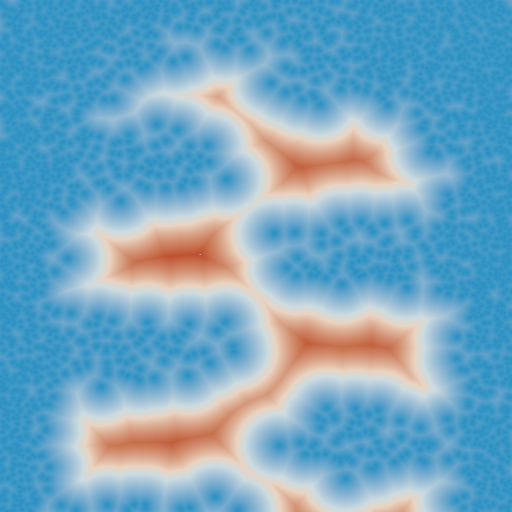
Euclidean Distance and Interpolation
A strong motivation for implementing Delaunay triangulations is to be able to furnish certain vector-to-raster operations.
EuclideanDistance allows us to build a raster where each tile cell contains
the distance from that cell to the closest point in a point set. This is
accomplished by rasterizing Voronoi cells using a distance function.
Euclidean distance tiles may be computed using either the
coordinates.euclideanDistance(re: RasterExtent) method extension or the
EuclideanDistanceTile(re: RasterExtent) apply method.
The other main class of vector-to-raster functions enabled by Delaunay
triangulations is linear interpolation of unstructured samples from some
function. We use the z-coordinate of our input points to store a Double
attribute for each point, and we rasterize the Delaunay triangles to produce
the final interpolation. The most obvious candidate is to use the
z-coordinates to indicate the elevation of points on the globe; the
rasterization of these values is a digital elevation map. This is the TIN
algorithm for DEM generation. Using this method, we would apply one of the
methods in geotrellis.raster.triangulation.DelaunayRasterizer.
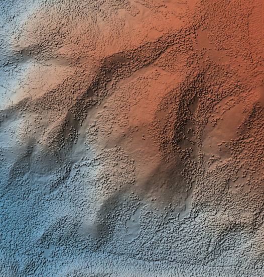
(The above image has been hillshaded to better show the detail in the elevation raster.)
The major advantage of using triangulations to interpolate is that it more gracefully handles areas with few or no samples, in contrast to a method such as inverse distance weighted interpolation, a raster-based technique. This is common when dealing with LiDAR samples that include water, which has spotty coverage due to the reflectance of water.
Distributed Computation
Among the design goals for this package was the need to handle extremely large
point sets—on the order of 100s of millions of points. To accomplish this
end, we opted for a distributed solution using Spark. Generally speaking,
this interface will require the user to cut the incoming point set according
to some LayoutDefinition into an RDD[(SpatialKey, Array[Coordinate])].
After triangulating each grid cell individually, facilities are provided to
join the results—though in certain cases, the results will not be as expected
(see Known Limitations below).
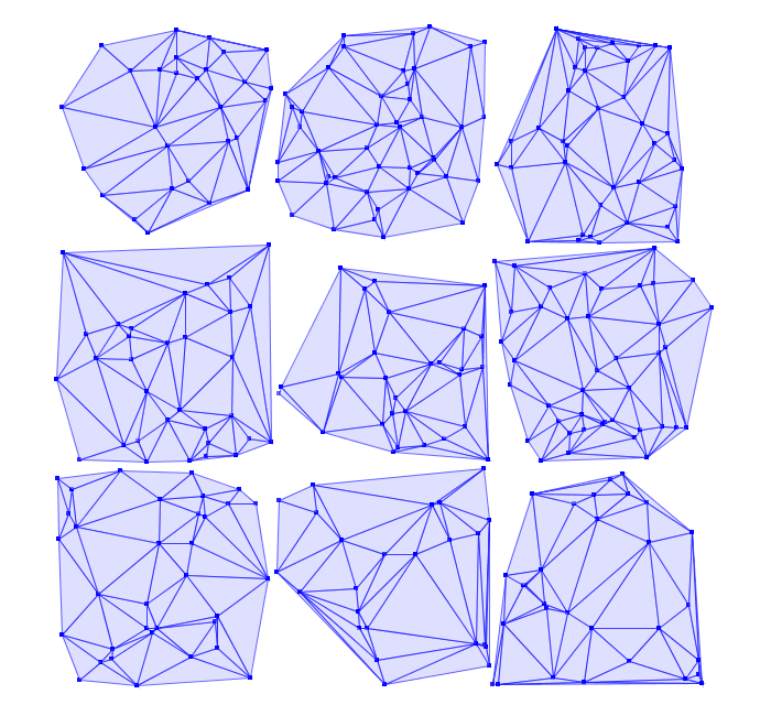
Given an RDD[(SpatialKey, DelaunayTriangulation)], one is meant to apply
the collectNeighbors() method to generate a map of nearby grid cells,
keyed by geotrellis.util.Direction. These maps are then taken as input to
StitchedDelaunay’s apply method. This will join a 3x3 neighborhood of
triangulations into a single triangulation by creating new triangles that fill
in the gaps between the component triangulations. For instance, if we begin
with the following collection of triangulations
The stitch operation creates the stitch triangles shown in red below:
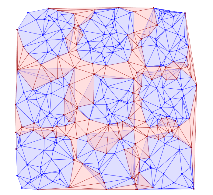
Notice that the stitch triangles overlap the base triangulations. This is
expected since not all the base triangles are Delaunay with respect to the
merged triangulation. Also keep in mind that in its current incarnation,
StitchedDelaunay instances’ triangles element contains only these fill
triangles, not the triangles of the base triangulations.
Because the interior of these base triangulations is often not needed, and they can be very large structures, to reduce shuffle volume during the distributed operation, we introduced the BoundaryDelaunay structure. These are derived from DelaunayTriangulations and an extent that entirely contains the triangulation, and inside which no points will be added in a subsequent stitch operation. The BoundaryDelaunay object will be a reduced mesh where the interior is empty. This is for context, as it is not recommended to interact with BoundaryDelaunay objects directly; that way madness lies. Nonetheless, it is an important operation to include due to the massive memory savings and reduced network traffic.
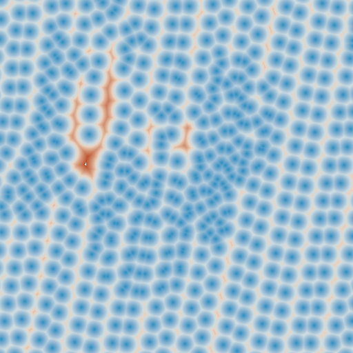
The immediate application of StitchedDelaunay is the ability to perform both
EuclideanDistance and interpolation tasks in a distributed context. We
provide the euclideanDistance(ld: LayoutDefinition) method extension
taking an RDD[(SpatialKey, Array[Coordinate])] to an RDD[(SpatialKey,
Tile)] (also available as the apply method on the EuclideanDistance
object in the geotrellis.spark.distance package). The following image is
one tile from such a Euclidean distance RDD. Notice that around the tile
boundary, we are seeing the influence of points from outside the tile’s
extent.
Keep in mind that one can rasterize non-point geometries as the basis for generic Euclidean distance computations, though this might start to be cost prohibitive if there are many polygonal areas in the input set.
Known Limitations
When designing this component, our aim was to handle the triangulation of dense, very large clouds of points with only small regions (relative to the layout definition) without any samples. That is to say, if there are occasional, isolated SpatialKeys that have no points, there is unlikely to be a problem. Multiple contiguous SpatialKeys with no points may cause problems. Specifically, in the case of Euclidean distance, if a tile has influence from outside the 3x3 area, there is likely to be errors. In the best case, there will be missing tiles, in the worst case, the Euclidean distance will simply be incorrect in certain areas.
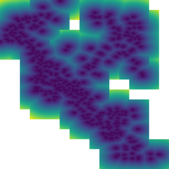
In this example, one can see that there are clear discontinuities in the
values along some tile boundaries. The upshot is that these erroneous tiles
are generated when (SpatialKey(c, r), Array.empty[Coordinate]) is included
in the source RDD. If the spatial key is simply not present, no tile will be
generated at that location, and the incidence of erroneous tiles will be
reduced, though not necessarily eliminated.
In cases where the point sample is small enough to be triangulated efficiently
on a single node, we recommend using
geotrellis.spark.distance.SparseEuclideanDistance to produce the Euclidean
distance tiles. This will produce the desired result.
Numerical Issues
When dealing with large, real-world point sets (particularly LiDAR data), one is likely to encounter triangulation errors that arise from numerical issues. We have done our best to be conscious of the numerical issues that surround these triangulation operations, including porting Jonathan Shewchuk’s robust predicates to Java, and offering some sensible numerical thresholds and tolerance parameters (not always accessible from the interface). Specifically, the DelaunayTriangulation object allows a distance threshold to be set, defining when two points are considered the same (only one will be retained, with no means of allowing the user to select which one).
The two most common errors will arise from points that are too close together for the numerical predicates to distinguish them, but too far apart to be considered a single point. Notably, during distributed tasks, this will produce stitch triangles which overlap the patches being joined. These errors arise from a known place in the code and can be dealt with by altering numerical thresholds, but there is currently no handle in the interface for setting these values.