Core Concepts
Geographical Information Systems (GIS), like any specialized field, has a wealth of jargon and unique concepts. When represented in software, these concepts can sometimes be skewed or expanded from their original forms. We give a thorough definition of many of the core concepts here, while referencing the Geotrellis objects and source files backing them.
This document aims to be informative to new and experienced GIS users alike. If GIS is brand, brand new to you, this document is a useful high level overview.
Glossary
The following is a non-exhaustive list of fundamental terms and their definitions that are important to understanding the function of Geotrellis. These definitions will be expanded upon in other sections of this document.
- Vector or Geometry: Structures built up by
connecting Points in space; includes
Points,Lines,Polygons. - Extent or Bounding Box: An axis aligned, rectangular region.
- Feature: A Geometry with some associated metadata.
- Cell: A single unit of data in some grid.
- Tile: A grid of numeric cells that represent some data on the Earth.
- Raster: A Tile with an Extent; places data over a specific region of the Earth.
- RDD: “Resilient Distributed Datasets” from Apache Spark. Can be thought of as a distributed Scala
Seq. - Key: Used to index into a grid of tiles.
- Layout Definition or Layout: A structure that relates keys to geographic locations and vice versa.
- Metadata or Layer Metadata: A descriptive structure that defines how to interpret a key-value store as a coherent single raster.
- Layer or Tile Layer: A combined structure
of tiles and keys in an
RDDwith metadata. Represents a very large raster in a distributed computing context. - Pyramid: A collection of layers, indexed by a zoom level, where each layer represents the same raster data at a different resolution. Essentially a quad tree of raster data where child nodes cover the same area at higher resolution as their parents.
- Catalog: A persistent store for tile layers and/or pyramids, storing both tiles and metadata.
System Organization
Core
The fundamental components of the Geotrellis system are rasters and vectors. Rasters are 2-dimensional, discrete grids of numerical data, much like matrices. Vectors are 2- (or sometimes 3-) dimensional collections of points that are connected together to form piecewise linear linestrings, polygons, and other compound structures.
Geotrellis is also tied to geographical application domains, and so these fundamental objects can be placed in a geographical context. Specifically, we can ascribe projections to the points in a geometry, and we can apply an extent to raster data to indicate the position and scope of the raster data.
Geotrellis provides a number of operations on these basic data types. One may reproject, resample, crop, merge, combine, and render raster data; vector data may be manipulated in some limited ways, but is mostly used to generate raster data.
The following packages contain the relevant code:
Distributed Processing
High resolution imagery on global, national, regional, or even local levels (depending on just how high of a resolution is used) is big. It’s too big to work with effectively on a single machine. Thus, Geotrellis provides the means to use rasters and vectors in a distributed context using Apache Spark.
To distribute data, it is necessary to supply some structure over which we can
organize smaller units of raster or vector data. Geotrellis leans on the
LayoutDefinition class to provide this structure. The idea is that a
region on the globe is specified (along with a projection), and a regular,
rectangular grid is overlaid on that region. Each grid cell is given a
spatial key, and so it is possible to associate a raster or vector to a given
grid cell. (Note that we may also use keys with a temporal component.) This
induces a tiled representation of an arbitrarily large layer of data.
Geotrellis provides utilities for coercing data into this gridded representation, for manipulating data within a tiled layer, and for storing processed layers to a variety of backends. Find implementations of these features in this package:
Storage Backends
Computations over large data are time consuming, so storage of results is important. Geotrellis mostly relies on distributed key-value stores. Once a layer is built (a set of uniform chunks of raster data keyed to a layout, with some additional metadata), it is possible to write these tiles out to a catalog. These preprocessed layers can then be read back rapidly, and used to support any number of applications.
The necessary componenents for storing and reading layers can be found in the following packages:
Method Extensions
Geotrellis utilizes a design pattern called method extensions wherein
Scala’s implicits system is used to patch additional functionality onto
existing classes. For example, for a raster value r, one may call
r.reproject(srcCRS, destCRS), even though the Raster class does not
define reproject directly.
Files in the source tree that have names of the form XxxxxMethods.scala
define capabilities that should be implemented by an implicit class, usually
found in the Implicits.scala file in the same directory. For a
MethodExtension[T] subclass implementing the foo() method, an object of type
T should be able to have foo() called on it.
Unfortunately, discoverability of valid method extensions is an ongoing
problem for Geotrellis as a whole. We are currently seeking better means for
documenting these features. In the meantime, perusing the source tree, and
using tab-completion in the REPL are workable solutions. Bear in mind,
however, that availability of method extensions is contingent on having
types that match the T parameter of the desired MethodExtension[T]
implementation.
Projections and Coordinate Systems
A fundamental component of a GIS system is the ability to specify projections
and perform transformations of points between various coordinate systems.
Contained in the geotrellis.proj4 package are the means to perform these
tasks.
Coordinate Reference Systems
As a means of describing geodetic coordinate systems, the
geotrellis.proj4.CRS class is provided. CRSs can be constructed by either
indicating the EPSG code using the CRS.fromEpsgCode object method, or by the
proj4 string using the CRS.fromString object method.
There are also a set of predefined CRS objects provided in
geotrellis.proj4. These include the standard WebMercator and LatLng
CRSs. Also included is ConusAlbers, giving the Albers equal area
projection for the continental United States (EPSG code 5070). Finally, UTM
zone CRS objects can be produced using the geotrellis.proj4.util.UTM.getZoneCrs method.
Transformations
To move coordinates between coordinate systems, it is necessary to build a
geotrellis.proj4.Transform object. These are built simply by supplying
the source CRS and the destination CRS. The result is a transformation
function with type (Double, Double) => (Double, Double).
Vector Data
Data in GIS applications often come in a geometric form. That is, one might encounter data describing, say, population by census region, or road networks. These are termed vector data sources. Geotrellis uses JTS geometries, but provides some code to make the use of that library’s classes easier and more idiomatic in a Scala context. We provide some added vector capabilities and tools to produce raster data from vector data. Vector data comes either as raw geometry, or as feature data—that is, geometry with associated data—and can be read from a variety of sources.
Geometries
Note
As of Geotrellis version 3, we have shifted to a direct reliance on JTS geometry classes. Interested users should consult the JTS documentation for details on that library’s capabilities and interface. However, we will give a rough overview of the basic vector classes here for convenience.
Note
In nearly all circumstances, it should not be necessary to
import org.locationtech.jts.geom._. Most of the types in that module
are mirrored by Geotrellis and will become available via:
import geotrellis.vector._
If some of the types provided by JTS are needed and not passed through by Geotrellis, it is important that the JTS imports are appropriately namespaced to avoid ambiguous references. We recommend using:
import org.locationtech.jts.{geom => jts}
JTS geometries are exclusively point sets and piecewise linear representations. A collection of points may be connected by a chain of linear segments into more complex shapes, and then aggregated into collections. The following is a list of available classes:
-
Representation of a 2-dimensional point in space.
-
More appropriately termed a polyline. A sequence of linear segments formed from a sequence of points, \([p_1, p_2, ..., p_n]\), where the \(i^\mathrm{th}\) line segment is the segment between \(p_i\) and \(p_{i+1}\). May be self-intersecting. May be open or closed (the latter meaning that \(p_1 = p_n\)).
-
A polygonal shape, possibly with holes. Formed from a single closed, simple (non-self-intersecting) polyline exterior, and zero or more closed, simple, mutually non-intersecting interior rings. Proper construction can be verified through the use of the
isValid()method. MultiPoint,MultiLineString,MultiPolygonEach of these classes represent a collection of the corresponding geometry type as a single object. This allows for multiple discrete geometries of a single type to be taken semantically as a single entity.
-
A container class for aggregating dissimilar geometries.
Geotrellis does add some facilities beyond those provided by JTS. Notably,
machinery to generate geometries is included. A global GeometryFactory is
available in geotrellis.vector.GeomFactory.factory that has been
configured through an application.conf (see the pureconfig
documentation) which set some global properties for that factory object. See
reference.conf for more details. The apply methods on Point,
LineString, Polygon, MultiPoint, MultiLineString,
MultiPolygon, and GeometryCollection in the geotrellis.vector
package rely internally on this global factory, and make creation of new
geometries easier.
Note
There is a bug in the Scala REPL which will prevent interactive use of the
apply methods on the basic geometry types when using console from SBT.
That is, when executing:
import geotrellis.vector._
val p1 = Point(0,0)
val p2 = Point(1,1)
you will encounter an error of the form error:
geotrellis.vector.Point.type does not take parameters.
For this reason, we provide the geotrellis.vector.JTS object, which
contains duplicates of the basic geometry types (e.g.,
geotrellis.vector.JTS.Point). The above code block can be modified
to:
import geotrellis.vector._
val p1 = JTS.Point(0,0)
val p2 = JTS.Point(1,1)
and it will work as expected.
This is a fix for a REPL bug, and thus is not required in compiled source.
In addition to these kinds of quality-of-life improvements, there are also
some major added features above and beyond the capabilities of JTS included in
geotrellis.vector. Specifically, we provide a fast Delaunay triangulator,
Kriging interpolation, and the means to perform projections between various
geodetic coordinate systems using proj4.
There is also the notable inclusion of GeoJSON input and output. Implicits
providing these capabilities in are found in geotrellis.vector.io._, and
after that import it becomes possible to call the toGeoJson method on any
Geometry:
import geotrellis.vector.io._
assert(Point(1,1).toGeoJson == """{"type":"Point","coordinates":[1.0,1.0]}""")
If you need to move from a geometry to a serialized representation or
vice-versa, take a look at the io directory’s contents. This naming
convention for input and output is common throughout Geotrellis. So if you’re
trying to get spatial representations in or out of your program, spend some
time seeing if the problem has already been solved. See
geotrellis.vector.io.json, geotrellis.vector.io.wkt, and
geotrellis.vector.io.wkb.
Finally, Geotrellis attempts to make working with geometries a bit more
idiomatic to Scala. Specifically, we prefer to pattern match on the results
of common geometric operations to catch missing logic during compile time,
rather than at some indeterminate point in the future as a run time error.
For instance, when working with intersections, if we use the standard JTS
intersection function, which returns a Geometry, we must then match on
the return type, including a wildcard case to catch the impossible outcomes
(e.g., polygons cannot result from a LineString intersection). It
is possible to forget some of the possible outcomes (e.g., the possibility of
a GeometryCollection result from a LineString-LineString intersection with
both linear and point components) and miss out on important program logic.
In order to provide these facilities, Geotrellis uses the method extensions
provided in geotrellis.vector.methods to furnish operators for difference,
union, and intersection that return some subclass of geotrellis.vector.GeometryResult that
participate in one of several algebraic data types which completely captures
the possible outcomes of the desired operation. We use the symbolic operators
-, |, and &, respectively, to denote the operations.
The results of these wrapper operators can be pattern matched completely without the need for a wildcard case, and will raise errors at compile time if a case is omitted.
import geotrellis.vector._

val line: LineString = ...
val poly: Polygon = ...

// Using JTS intersection method
line.intersection(poly) match {
  case l: LineString => ...
  case _ => throw new Exception("Unhandled")
}

// Using Geotrellis wrapper
line & poly match {
  case NoResult => ...
  case PointResult(p) => ...
  case LineStringResult(l) => ...
  case GeometryCollectionResult(gc) => ...
}
It is also possible to work with the result types directly. To extract
results from these result wrappers, use the as[G <: Geometry] function
which either returns Some(G) or None. When using as[G <:
Geometry], be aware that it isn’t necessarily the case that the
geotrellis.vector.GeometryResult object may not be convertable to the chosen G. For
example, a PointGeometryIntersectionResult.as[Polygon] will always
return None. For example, a Point/Point intersection has the type
PointOrNoResult. From this we can deduce that it is either a Point
underneath or else nothing:
val p1: Point = Point(0, 0)
val p2: Point = p1
(p1 & p2).as[Point] match {
  case Some(_) => println("A Point!")
  case None => println("Sorry, no result.")
}
This snippet yields “A Point!” Please see Results.scala for complete
details on the various result types.
Extents
Geotrellis makes common use of the Extent class. This class represents an
axis-aligned bounding box, where the extreme values are given as
Extent(min_x, min_y, max_x, max_y). Note that Extents are not
Geometry instances, nor are they JTS Envelope``s. They can be coerced
to a ``Polygon using the toPolygon method or to an Envelope using
the jtsEnvelope method.
Projected Geometries
Note that there is no generally-accepted means to mark the projection of a
geometry, so it is incumbent on the user to keep track of and properly coerce
geometries into the correct projections. However, the
geotrellis.vector.reproject package provides the reproject method
extension for performing this task.
Extents, on the other hand, can be wrapped in a ProjectedExtent
instance. These are useful for designating the geographical scope of a
raster, for example.
Features
To associate some arbitrary data with a vector object, often for use in tasks
such as rasterization, use the Feature[G <: Geometry, D] container class,
or one of its subclasses. For example:
abstract class Feature[D] {
  type G <: Geometry
  val geom: G ; val data: D
}

case class PointFeature[D](geom: Point, data: D) extends Feature[D] {type G = Point}
Implicit method extensions exist that will allow, for instance, rasterize
to be called on a Feature to create a raster where the pixels covered by
the geometry are assigned the value of of the feature’s data.
Raster Data
Tiles and Rasters
The geotrellis.raster module provides primitive datatypes to represent two
dimensional, gridded numerical data structures, and the methods to manipulate
them in a GIS context. These raster objects resemble sequences of numerical
sequences like the following (this array of arrays is like a 3x3 tile):
// not real syntax
val myFirstTile = [[1,1,1],[1,2,2],[1,2,3]]
/** It probably looks more like your mental model if we stack them up:
  * [[1,1,1],
  *  [1,2,2],
  *  [1,2,3]]
  */
In the raster module of GeoTrellis, raster data is not represented by
simple arrays, but rather as subclasses of Tile. That class is more
powerful than a simple array representation, providing many useful
operators. Here’s an incomplete list of the types of things on offer:
- Mapping transformations of arbitrary complexity over the constituent cells
- Carrying out operations (side-effects) for each cell
- Querying a specific tile value
- Rescaling, resampling, cropping
Working with Cell Values
Tiles contain numerical data. These can be of the form of integers,
floats, doubles, and so forth. And even though Scala has generic types,
Geotrellis does not implement Tile[V] for performance reasons, since the
Java compiler will liberally sprinkle box/unbox commands all through the code
to support the genericity, which greatly increase runtime and space usage.
Instead, Geotrellis uses macros to implement a different system of cell types. This preserves speed while maintaining flexibility of data types, with only small compromises in the API. These cell types may also represent no data, that is, a special value can be assigned to represent a missing value. This does require sacrificing a value from the range of possible inputs, but eliminates the problems of boxed types, such as Option. (Note, this means that bit-valued cells cannot have no data values.)
The various cell types are defined as follows:
| No NoData | Constant NoData | User Defined NoData | |
|---|---|---|---|
| BitCells | BitCellType |
N/A | N/A |
| ByteCells | ByteCellType |
ByteConstantNoDataCellType |
ByteUserDefinedNoDataCellType |
| UbyteCells | UByteCellType |
UByteConstantNoDataCellType |
UByteUserDefinedNoDataCellType |
| ShortCells | ShortCellType |
ShortConstantNoDataCellType |
ShortUserDefinedNoDataCellType |
| UShortCells | UShortCellType |
UShortConstantNoDataCellType |
UShortUserDefinedNoDataCellType |
| IntCells | IntCellType |
IntConstantNoDataCellType |
IntUserDefinedNoDataCellType |
| FloatCells | FloatCellType |
FloatConstantNoDataCellType |
FloatUserDefinedNoDataCellType |
| DoubleCells | DoubleCellType |
DoubleConstantNoDataCellType |
DoubleUserDefinedNoDataCellType |
The three rightmost columns give the CellTypes that would be used to
represent (1) data without a NoData value, (2) data using a default
NoData value, and (3) data where the user specifies the value used for the
NoData value. User defined NoData CellTypes require a constructor to
provide the NoData value.
A caveat: The single most noticeable compromise of this system is that
float- and double-valued cell types must be treated differently using
functions such as getDouble, setDouble, and mapDouble, provided by
the tile classes.
Now, some examples:
/** Here's an array we'll use to construct tiles */
val myData = Array(42, 1, 2, 3)

/** The GeoTrellis-default integer CellType
 *   Note that it represents `NoData` values with the smallest signed
 *   integer possible with 32 bits (Int.MinValue or -2147483648).
 */
val defaultCT = IntConstantNoDataCellType
val normalTile = IntArrayTile(myData, 2, 2, defaultCT)

/** A custom, 'user defined' NoData CellType for comparison; we will
 *   treat 42 as NoData for this one rather than Int.MinValue
 */
val customCellType = IntUserDefinedNoDataCellType(42)
val customTile = IntArrayTile(myData, 2, 2, customCellType)

/** We should expect that the first (default celltype) tile has the value 42 at (0, 0)
 *   This is because 42 is just a regular value (as opposed to NoData)
 *   which means that the first value will be delivered without surprise
 */
assert(normalTile.get(0, 0) == 42)
assert(normalTile.getDouble(0, 0) == 42.0)

/** Here, the result is less obvious. Under the hood, GeoTrellis is
 *   inspecting the value to be returned at (0, 0) to see if it matches our
 *   `NoData` policy and, if it matches (it does, we defined NoData as
 *   42 above), return Int.MinValue (no matter your underlying type, `get`
 *   on a tile will return an `Int` and `getDouble` will return a `Double`).
 *
 *   The use of Int.MinValue and Double.NaN is a result of those being the
 *   GeoTrellis-blessed values for NoData - below, you'll find a chart that
 *   lists all such values in the rightmost column
 */
assert(customTile.get(0, 0) == Int.MinValue)
assert(customTile.getDouble(0, 0) == Double.NaN)
One final point is worth making in the context of CellType
performance: the Constant types are able to depend upon macros which
inline comparisons and conversions. This minor difference can certainly
be felt while iterating through millions and millions of cells. If
possible, Constant NoData values are to be preferred. For
convenience’ sake, we’ve attempted to make the GeoTrellis-blessed
NoData values as unobtrusive as possible a priori.
- Notes:
If attempting to convert between
CellTypes, see this note onCellTypeconversions.)Lower-precision cell types will translate into smaller tiles. Consider the following:
Bits / Cell 512x512 Raster (mb) Range (inclusive) GeoTrellis NoData Value BitCells 1 0.032768 [0, 1] N/A ByteCells 8 0.262144 [-128, 128] -128 ( Byte.MinValue)UbyteCells 8 0.262144 [0, 255] 0 ShortCells 16 0.524288 [-32768, 32767] -32768 ( Short.MinValue)UShortCells 16 0.524288 [0, 65535] 0 IntCells 32 1.048576 [-2147483648, 2147483647] -2147483648 ( Int.MinValue)FloatCells 32 1.048576 [-3.40E38, 3.40E38] Float.NaN DoubleCells 64 2.097152 [-1.79E308, 1.79E308] Double.NaN Also note the range and default no data values (
ConstantNoDataCellTypes).The limits of expected return types (see above table) are used by macros to squeeze as much speed out of the JVM as possible. Check out our macros docs for more on our use of macros like
isDataandisNoData.
Building Your Own Tiles
An easy place to begin with building a tile is through one of the following two classes:
abstract class IntArrayTile(
  val array: Array[Int],
  cols: Int,
  rows: Int
) extends MutableArrayTile { ... }

abstract class DoubleArrayTile(
  val array: Array[Double],
  cols: Int,
  rows: Int
) extends MutableArrayTile { ... }
These constructors allow for an Int- or Double-valued tile to be
created with specific content. However, the object methods associated with
these classes contain most of the useful constructors. Notably, the apply
method One may also enjoy using the empty, fill, and ofDim object
methods to create new tiles. For these methods,
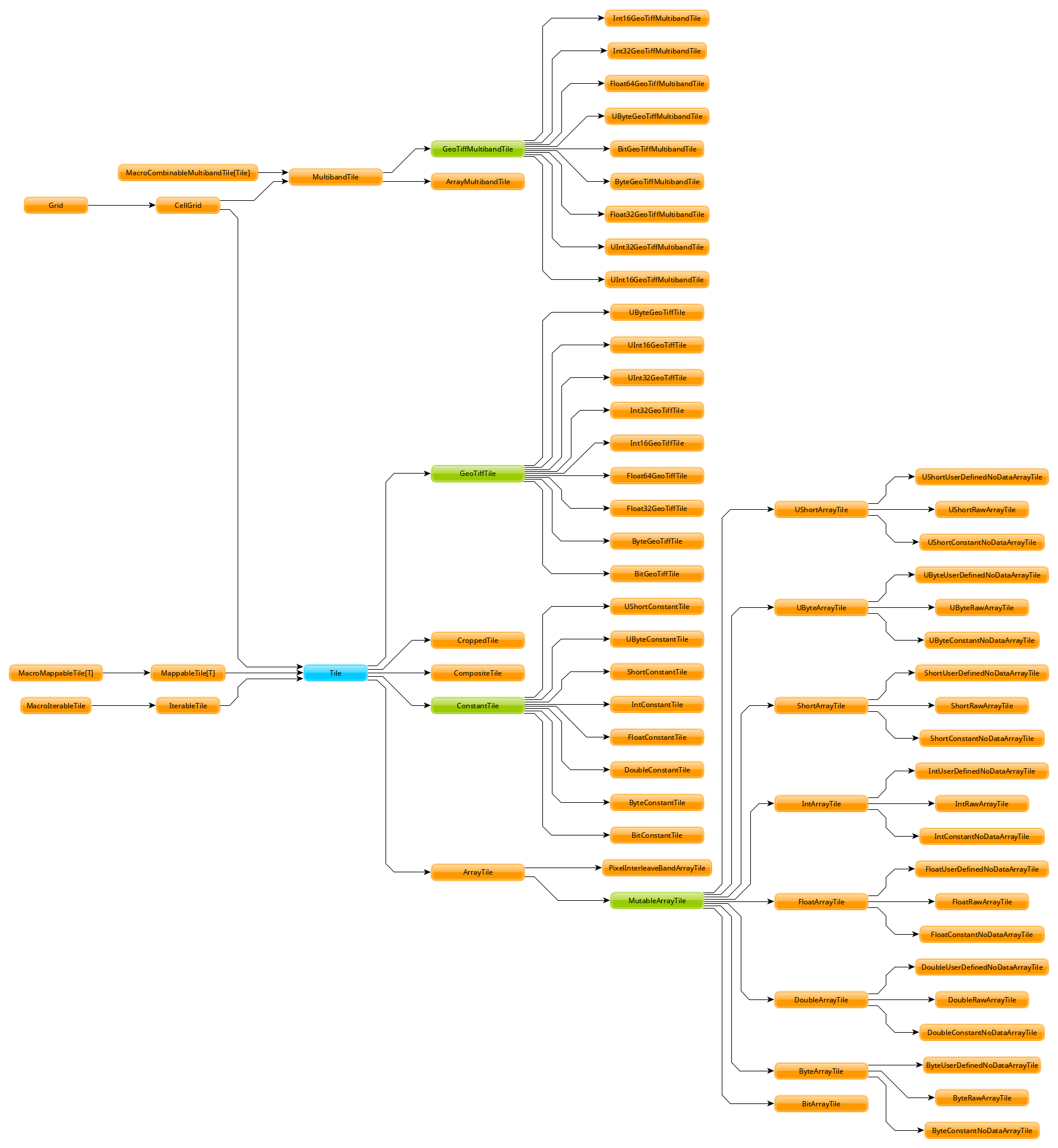
Tile Inheritance Structure
We can consider the inheritance pathway of IntArrayTile to get a feel for
the class structure. Note that each listed class is a descendant of the
previous class.
-
A
Serializableinstance giving row and column dimensions. -
Adds
cellTypeto Grid.CellGridforms the minimum requirement for many algorithms. -
Provides the basic infrastructure for accessing the content of a tile (
getandgetDouble). -
Allows conversion from tiles to arrays.
-
Provides the means to change the values in a tile (
setandsetDouble). -
The implementation of
MutableArrayTilefor discrete data types.NOTE There is a long-standing bug in the Tile hierarchy where calling
mutableon an ArrayTile instance does not create a copy of the original immutable tile, but simply creates a mutable version from the same underlying buffer. Changes to the result of a call tomutablewill change the original as well.
Rasters
A raster is a general category of data, consisting of values laid out on a
regular grid, but in GIS, it carries the double meaning of a tile with
location information. The location information is represented by an Extent.
This is almost always meant when we use the proper term Raster in the
context of Geotrellis code.
The following REPL session constructs a simple Raster:
import geotrellis.raster._
import geotrellis.vector._

scala> IntArrayTile(Array(1,2,3),1,3)
res0: geotrellis.raster.IntArrayTile = IntArrayTile([S@338514ad,1,3)

scala> IntArrayTile(Array(1,2,3),3,1)
res1: geotrellis.raster.IntArrayTile = IntArrayTile([S@736a81de,3,1)

scala> IntArrayTile(Array(1,2,3,4,5,6,7,8,9),3,3)
res2: geotrellis.raster.IntArrayTile = IntArrayTile([I@5466441b,3,3)

scala> Extent(0, 0, 1, 1)
res4: geotrellis.vector.Extent = Extent(0.0,0.0,1.0,1.0)

scala> Raster(res2, res4)
res5: geotrellis.raster.Raster = Raster(IntArrayTile([I@7b47ab7,1,3),Extent(0.0,0.0,1.0,1.0))

scala> res0.asciiDraw()
res3: String =
"    1
     2
     3
"

scala> res2.asciiDraw()
res4: String =
"    1     2     3
     4     5     6
     7     8     9
"
Tile Hierarchy
For the sake of completeness, the following tile hierarchy is presented:
The Tile trait has operations you’d expect for traversing and
transforming the contents of the tiles, like:
map: (Int => Int) => Tileforeach: (Int => Unit) => Unitcombine: Tile => ((Int, Int) => Int) => Tilecolor: ColorMap => Tile
As discussed above, the Tile interface carries information about how big
it is and what its underlying Cell Type is:
cols: Introws: IntcellType: CellType
Layouts and Tile Layers
The core vector and raster functionality thus far described stands on its own for small scale applications. But, as mentioned, Geotrellis is intended to work with big data in a distributed context. For this, we rely on Apache Spark’s resilient distributed dataset (RDD). RDDs of both raster and vector data are naturally supported by Geotrellis, but some new concepts are required to integrate this abstraction for distributed processing.
For most applications, the data of interest must be keyed to a layout to give
the content of an RDD—which is usually a collection of key-value pairs (i.e.,
RDD[(K, V)])—a consistent interpretation as a cohesive raster. In such an
RDD, the key type, K, is one of TemporalKey, SpatialKey, or
SpaceTimeKey. The latter two key types obviously contain spatial data
(declared in context bounds as [K: SpatialComponent], where values of such
a type K can have their spatial component extracted using the
getComponent[SpatialKey] extension method), which is used to identify a
region in space.
The geotrellis.spark.tiling.LayoutDefinition class is used to describe how
SpatialKeys map to regions in space. The LayoutDefinition is a
GridExtent subclass defined with an Extent and CellSize. The
Extent is subdivided into a grid of uniform, rectangular regions. The
size and number of the sub-regions is determined using the CellSize of the
LayoutDefinition, and then the pixel dimensions of the constituent tiles.
The sub-regions are then assigned a SpatialKey with the (0, 0)
position corresponding to the upper-left corner of the extent; the x
coordinate increases toward the right, and the y coordinate increases moving
down (into lower latitude values, say).
Thus far, we’ve described how an RDD[(K, V)] plus a LayoutDefinition
can be used to represent a large, distributed raster (when [K:
SpatialComponent]). To solidify this notion, Geotrellis has a notion of a
Tile Layer, which is defined as RDD[(K, V)] with Metadata[M]. The M
type is usually represented by a TileLayerMetadata[K] object. These
metadata, provide a LayoutDefinition plus a CRS, CellType, and
bounds for the keys found in the RDD.
Note: The easiest means to represent a tile layer is with a
ContextRDDobject.Note: Geotrellis offers many method extensions that operate on tile layers, but it is occasionally necessary to explicitly declare the types of
V,K, andMto access those methods.
The following figure summarizes the structure of a tile layer and its constituent parts:
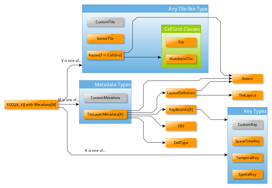
In this diagram:
CustomTile,CustomMetadata, andCustomKeydon’t exist, they represent types that you could write yourself for your application.- The
Kseen in several places is the sameK. - The type
RDD[(K, V)] with Metadata[M]is a Scala Anonymous Type. In this case, it meansRDDfrom Apache Spark with extra methods injected from theMetadatatrait. This type is sometimes aliased in GeoTrellis asContextRDD. RDD[(K, V)]resembles a ScalaSeq[(K, V)], but also has furtherMap-like methods injected by Spark when it takes this shape. See Spark’s PairRDDFunctions Scaladocs for those methods. Note: UnlikeMap, theKs here are not guaranteed to be unique.
TileLayerRDD
Geotrellis defines a type alias for a common variant of a tile layer,
RDD[(K, V)] with Metadata[M], as follows:
type TileLayerRDD[K] = RDD[(K, Tile)] with Metadata[TileLayerMetadata[K]]
This type represents a grid (or cube!) of Tiles on the earth,
arranged according to some K. Features of this grid are:
- Grid location
(0, 0)is the top-leftmostTile. - The
Tiles exist in some CRS. InTileLayerMetadata, this is kept track of with an actualCRSfield. - In applications,
Kis mostlySpatialKeyorSpaceTimeKey.
Keys and Key Indexes
Keys
As mentioned in the Tile Layers section, grids (or
cubes) of Tiles on the earth are organized by keys. This key,
often refered to generically as K, is typically a SpatialKey or
a SpaceTimeKey:
case class SpatialKey(col: Int, row: Int)

case class SpaceTimeKey(col: Int, row: Int, instant: Long)
It is also possible to define custom key types.
Reminder: Given a layout over someExtent,SpatialKey(0, 0)would index the top-leftmostTilein the grid covering that extent.
When doing Layer IO, certain optimizations can be performed if we know
that Tiles stored near each other in a filesystem or database
(like Accumulo or HBase) are also spatially-close in the grid they’re
from. To make such a guarantee, we use a KeyIndex.
Key Indexes
A KeyIndex is a GeoTrellis trait that represents Space Filling
Curves. They are a
means by which to translate multi-dimensional indices into a
single-dimensional one, while maintaining spatial locality. In GeoTrellis,
we use these chiefly when writing Tile Layers to one of our Tile Layer
Backends.
Although KeyIndex is often used in its generic trait form, we
supply three underlying implementations.
Z-Curve

The Z-Curve is the simplest KeyIndex to use (and implement). It can
be used with both SpatialKey and SpaceTimeKey.
val b0: KeyBounds[SpatialKey] = ... /* from `TileLayerRDD.metadata.bounds` */
val b1: KeyBounds[SpaceTimeKey] = ...

val i0: KeyIndex[SpatialKey] = ZCurveKeyIndexMethod.createIndex(b0)
val i1: KeyIndex[SpaceTimeKey] = ZCurveKeyIndexMethod.byDay().createIndex(b1)

val k: SpatialKey = ...
val oneD: Long = i0.toIndex(k) /* A SpatialKey's 2D coords mapped to 1D */
Hilbert

Another well-known curve, available for both SpatialKey and
SpaceTimeKey.
val b: KeyBounds[SpatialKey] = ...

val index: KeyIndex[SpatialKey] = HilbertKeyIndexMethod.createIndex(b)
Index Resolution Changes Index Order
Changing the resolution (in bits) of the index causes a rotation and/or reflection of the points with respect to curve-order. Take, for example the following code (which is actually derived from the testing codebase):
HilbertSpaceTimeKeyIndex(SpaceTimeKey(0,0,y2k), SpaceTimeKey(2,2,y2k.plusMillis(1)),2,1)
The last two arguments are the index resolutions. If that were changed to:
HilbertSpaceTimeKeyIndex(SpaceTimeKey(0,0,y2k), SpaceTimeKey(2,2,y2k.plusMillis(1)),3,1)
The index-order of the points would be different. The reasons behind
this are ultimately technical, though you can imagine how a naive
implementation of an index for, say, a 10x10 matrix (in terms of 100
numbers) would need to be reworked if you were to change the number of
cells (100 would no longer be enough for an 11x11 matrix and the pattern
for indexing you chose may no longer make sense). Obviously, this is
complex and beyond the scope of GeoTrellis’ concerns, which is why we
lean on Google’s uzaygezen library.
Beware the 62-bit Limit
Currently, the spatial and temporal resolution required to index the points, expressed in bits, must sum to 62 bits or fewer.
For example, the following code appears in
HilbertSpaceTimeKeyIndex.scala:
@transient
lazy val chc = {
  val dimensionSpec =
    new MultiDimensionalSpec(
      List(
        xResolution,
        yResolution,
        temporalResolution
      ).map(new java.lang.Integer(_))
    )
}
where xResolution, yResolution and temporalResolution are
numbers of bits required to express possible locations in each of those
dimensions. If those three integers sum to more than 62 bits, an error
will be thrown at runtime.
Row Major
Row Major is only available for SpatialKey, but provides the fastest
toIndex lookup of the three curves. It doesn’t however, give good
locality guarantees, so should only be used when locality isn’t as
important to your application.
val b: KeyBounds[SpatialKey] = ...

val index: KeyIndex[SpatialKey] = RowMajorKeyIndexMethod.createIndex(b)
Pyramids
In practice, many map applications have an interactive component. Interaction often takes the form of scrolling around the map to a desired location and “zooming in”. This usage pattern implies a need for levels of detail. That is, if we start with a layer with a cell size of 10 meters on a side, say, then viewing the whole continental US would require a raster in the neighborhood of 400,000 x 250,000 pixels, and most of that information would never be seen.
The common solution for this problem is to build a level of detail pyramid, that is, we generate from the base layer a series of less resolute layers, with larger cell size, but a smaller number of pixels. Each layer of the pyramid is called a zoom level.
It is typical for web maps to employ power of two zoom levels, which is to say that the map should double its cell size (halve its resolution) at each successive zoom level. In terms of tile layers, this means that we will end up grouping each layer’s tiles into 2x2 clusters, and merge these chunks into a single tile in the successive layer. In short, we are creating a quad tree where each interior node has an associated tile formed from the resampled and merged tiles of its children.
Note: In a Geotrellis pyramid, each level of the pyramid is a layer with its associated metadata.
To build a pyramid, Geotrellis provides the
geotrellis.spark.pyramid.Pyramid class. Consult that documentation for
usage.
Zoom Levels and Layout Schemes
The generation of a pyramid is the generation of a quadtree, but that is not
entirely sufficient, because it is necessary to “contextualize” a tree level.
In some cases, the layer on which the pyramid is based has a well-defined
LayoutDefinition that is significant to the application. In those cases,
we simply build the pyramid. In other cases, we need to generate
LayoutDefinitions that conform to the application’s demand. This is the
job of a geotrellis.spark.tiling.LayoutScheme.
A LayoutScheme sets the definition of a zoom level. Given an extent and a
cell size, the LayoutScheme will provide an integer zoom level and the
layout definition for that canonical zoom level (the levelFor() method).
Above and beyond that, a LayoutScheme allows for the navigation between
adjacent zoom levels with the zoomIn() and zoomOut() methods.
There are two primary modes of setting zoom levels, which can be thought of as
local and global. A local method is akin to starting with a
LayoutDefinition and assigning an arbitrary zoom number to it. The leaf
nodes of the pyramid’s quad tree are rooted at this level, and subsequent zoom
levels (lower resolution levels) are generated through power of two
reductions. Use the geotrellis.spark.tiling.LocalLayoutScheme class for this purpose.
Note: The user must specify the numerical value of the initial zoom level when using aLocalLayoutScheme.
Global layout schemes, on the other hand, have a predefined structure. These
schemes start with a global extent, which each CRS defines. A tile
resolution is set, which defines the cell size at zoom level 0—that is, global
layout schemes are defined by having one tile which covers the world extent
completely at zoom 0. That cell size is then halved at the next highest (more
resolute) zoom level. For historical reasons, global schemes are called geotrellis.spark.tiling.ZoomedLayoutSchemes
Note: the global layout scheme defined here establishes a zoom and spatial key layout that is used by many prevalent web map tile serving standards such as TMS.
Catalogs & Tile Layer IO
There is a significant amount of embodied effort in any given layer or pyramid, thus it is a common use case to want to persist these layers to some storage back end. A set of saved layers under a common location with some metadata store is called a catalog in Geotrellis parlance. There can be multiple different pyramids in a catalog, and the metadata can be extended for a particular use case. This section explains the components of a catalog and how to perform IO between an application and a catalog.
Layer IO requires a Tile Layer Backend. Each
backend has an AttributeStore, a LayerReader, and a
LayerWriter.
An example using the file system backend:
import geotrellis.spark._
import geotrellis.spark.io._
import geotrellis.spark.io.file._

val catalogPath: String = ...  /* Some location on your computer */

val store: AttributeStore = FileAttributeStore(catalogPath)

val reader = FileLayerReader(store)
val writer = FileLayerWriter(store)
Writing an entire layer:
/* Zoom level 13 */
val layerId = LayerId("myLayer", 13)

/* Produced from an ingest, etc. */
val rdd: TileLayerRDD[SpatialKey] = ...

/* Order your Tiles according to the Z-Curve Space Filling Curve */
val index: KeyIndex[SpatialKey] = ZCurveKeyIndexMethod.createIndex(rdd.metadata.bounds)

/* Returns `Unit` */
writer.write(layerId, rdd, index)
Reading an entire layer:
/* `.read` has many overloads, but this is the simplest */
val sameLayer: TileLayerRDD[SpatialKey] = reader.read(layerId)
Querying a layer (a “filtered” read):
/* Some area on the earth to constrain your query to */
val extent: Extent = ...

/* There are more types that can go into `where` */
val filteredLayer: TileLayerRDD[SpatialKey] =
  reader.query(layerId).where(Intersects(extent)).result
Catalog Organization
Our Landsat Tutorial produces a
simple single-pyramid catalog on the filesystem at data/catalog/ which
we can use here as a reference. Running tree -L 2 gives us a view of the
directory layout:
.
├── attributes
│   ├── landsat__.__0__.__metadata.json
│   ├── landsat__.__10__.__metadata.json
│   ├── landsat__.__11__.__metadata.json
│   ├── landsat__.__12__.__metadata.json
│   ├── landsat__.__13__.__metadata.json
│   ├── landsat__.__1__.__metadata.json
│   ├── landsat__.__2__.__metadata.json
│   ├── landsat__.__3__.__metadata.json
│   ├── landsat__.__4__.__metadata.json
│   ├── landsat__.__5__.__metadata.json
│   ├── landsat__.__6__.__metadata.json
│   ├── landsat__.__7__.__metadata.json
│   ├── landsat__.__8__.__metadata.json
│   └── landsat__.__9__.__metadata.json
└── landsat
    ├── 0
    ├── 1
    ├── 10
    ├── 11
    ├── 12
    ├── 13
    ├── 2
    ├── 3
    ├── 4
    ├── 5
    ├── 6
    ├── 7
    ├── 8
    └── 9

16 directories, 14 files
The children of landsat/ are directories, but we used -L 2 to hide
their contents. They actually contain thousands of Tile files, which are
explained below.
Metadata
The metadata JSON files contain familiar information:
$ jshon < lansat__.__6__.__metadata.json
  [
    {
      "name": "landsat",
      "zoom": 6
    },
    {
      "header": {
        "format": "file",
        "keyClass": "geotrellis.spark.SpatialKey",
        "valueClass": "geotrellis.raster.MultibandTile",
        "path": "landsat/6"
      },
      "metadata": {
        "extent": {
          "xmin": 15454940.911194608,
          "ymin": 4146935.160646211,
          "xmax": 15762790.223459147,
          "ymax": 4454355.929947533
        },
        "layoutDefinition": { ... }
      },
      ... // more here
      "keyIndex": {
        "type": "zorder",
        "properties": {
          "keyBounds": {
            "minKey": { "col": 56, "row": 24 },
            "maxKey": { "col": 57, "row": 25 }
          }
        }
      },
      ... // more here
    }
  ]
Of note is the header block, which tells GeoTrellis where to look for
and how to interpret the stored Tiles, and the keyIndex block
which is critical for reading/writing specific ranges of tiles. For more
information, see our section on Key Indexes.
As we have multiple storage backends, header can look different. Here’s
an example for a Layer ingested to S3:
... // more here
"header": {
   "format": "s3",
   "key": "catalog/nlcd-tms-epsg3857/6",
   "keyClass": "geotrellis.spark.SpatialKey",
   "valueClass": "geotrellis.raster.Tile",
   "bucket": "azavea-datahub"
 },
 ... // more here
Tiles
From above, the numbered directories under landsat/ contain serialized
Tile files.
$ ls
attributes/  landsat/
$ cd landsat/6/
$ ls
1984  1985  1986  1987
$ du -sh *
12K     1984
8.0K    1985
44K     1986
16K     1987
Note
These Tile files are not images, but can be rendered by
GeoTrellis into PNGs.
Notice that the four Tile files here have different sizes. Why might
that be, if Tiles are all Rasters of the same dimension? The answer is
that a Tile file can contain multiple tiles. Specifically, it is a
serialized Array[(K, V)] of which Array[(SpatialKey, Tile)] is a
common case. When or why multiple Tiles might be grouped into a single
file like this is the result of the Space Filling Curve
algorithm applied during ingest.
Separate Stores for Attributes and Tiles
The real story here is that layer attributes and the Tiles themselves
don’t need to be stored via the same backend.
Indeed, when instantiating a Layer IO class like S3LayerReader, we notice
that its AttributeStore parameter is type-agnostic:
class S3LayerReader(val attributeStore: AttributeStore)
So it’s entirely possible to store your metadata with one service and your
tiles with another. Due to the header block in each Layer’s metadata,
GeoTrellis will know how to fetch the Tiles, no matter how they’re
stored. This arrangement could be more performant/convenient for you,
depending on your architecture.
Map Algebra
Map Algebra is the name given by Dana Tomlin to a method of manipulating and transforming raster data. There are many references on map algebra, including Tomlin’s book, so we will only give a brief introduction here. GeoTrellis follows Tomlin’s vision of map algebra operations, although there are many operations that fall outside of the realm of Map Algebra that it also supports.
Map Algebra operations fall into 3 general categories:
Local Operations
Local operations are ones that only take into account the information of on cell at a time. In the animation above, we can see that the blue and the yellow cell are combined, as they are corresponding cells in the two tiles. It wouldn’t matter if the tiles were bigger or smaller - the only information necessary for that step in the local operation is the cell values that correspond to each other. A local operation happens for each cell value, so if the whole bottom tile was blue and the upper tile were yellow, then the resulting tile of the local operation would be green.
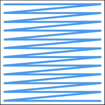
Focal Operations
Focal operations take into account a cell, and a neighborhood around that
cell. A neighborhood can be defined as a square of a specific size, or
include masks so that you can have things like circular or wedge-shaped
neighborhoods. In the above animation, the neighborhood is a 5x5 square
around the focal cell. The focal operation in the animation is a
focalSum. The focal value is 0, and all of the other cells in the focal
neighborhood; therefore the cell value of the result tile would be 8 at the
cell corresponding to the focal cell of the input tile. This focal operation
scans through each cell of the raster. You can imagine that along the
border, the focal neighborhood goes outside of the bounds of the tile; in
this case the neighborhood only considers the values that are covered by the
neighborhood. GeoTrellis also supports the idea of an analysis area, which
is the GridBounds that the focal operation carries over, in order to support
composing tiles with border tiles in order to support distributed focal
operation processing.
Zonal Operations
Zonal operations are ones that operate on two tiles: an input tile, and a
zone tile. The values of the zone tile determine what zone each of the
corresponding cells in the input tile belong to. For example, if you are
doing a zonalStatistics operation, and the zonal tile has a distribution
of zone 1, zone 2, and zone 3 values, we will get back the statistics such
as mean, median and mode for all cells in the input tile that correspond to
each of those zone values.
Using Map Algebra Operations
Map Algebra operations are defined as implicit methods on Tile or
Traversable[Tile], which are imported with import
geotrellis.raster._.
import
geotrellis.raster._
val tile1: Tile = ???
val tile2: Tile = ???
// If tile1 and tile2 are the same dimensions, we can combine
// them using local operations
tile1.localAdd(tile2)
// There are operators for some local operations.
// This is equivalent to the localAdd call above
tile1 + tile2
// There is a local operation called "reclassify" in literature,
// which transforms each value of the function.
// We actually have a map method defined on Tile,
// which serves this purpose.
tile1.map { z => z + 1 } // Map over integer values.
tile2.mapDouble { z => z + 1.1 } // Map over double values.
tile1.dualMap({ z => z + 1 })({ z => z + 1.1 }) // Call either the integer value or double version, depending on cellType.
// You can also combine values in a generic way with the combine funciton.
// This is another local operation that is actually defined on Tile directly.
tile1.combine(tile2) { (z1, z2) => z1 + z2 }
The following packages are where Map Algebra operations are defined in GeoTrellis:
- geotrellis.raster.mapalgebra.local defines operations which act on a cell without regard to its spatial relations. Need to double every cell on a tile? This is the module you’ll want to explore.
- geotrellis.raster.mapalgebra.focal defines operations which focus on two-dimensional windows (internally referred to as neighborhoods) of a raster’s values to determine their outputs.
- geotrellis.raster.mapalgebra.zonal defines operations which apply over a zones as defined by corresponding cell values in the zones raster.
Conway’s Game of Life can be seen as a
focal operation in that each cell’s value depends on neighboring cell
values. Though focal operations will tend to look at a local region of this
or that cell, they should not be confused with the operations which live in
geotrellis.raster.local - those operations describe transformations over
tiles which, for any step of the calculation, need only know the input value
of the specific cell for which it is calculating an output (e.g.
incrementing each cell’s value by 1).
Vector Tiles
Invented by Mapbox, VectorTiles are a combination of the ideas of finite-sized tiles and vector geometries. Mapbox maintains the official implementation spec for VectorTile codecs. The specification is free and open source.
VectorTiles are advantageous over raster tiles in that:
- They are typically smaller to store
- They can be easily transformed (rotated, etc.) in real time
- They allow for continuous (as opposed to step-wise) zoom in Slippy Maps.
Raw VectorTile data is stored in the protobuf format. Any codec implementing the spec must decode and encode data according to this .proto schema.
GeoTrellis provides the geotrellis-vectortile module, a
high-performance implementation of Version 2.1 of the VectorTile
spec. It features:
- Decoding of Version 2 VectorTiles from Protobuf byte data into useful Geotrellis types.
- Lazy decoding of Geometries. Only parse what you need!
- Read/write VectorTile layers to/from any of our backends.
As of 2016 November, ingests of raw vector data into VectorTile sets aren’t yet possible.
Small Example
import geotrellis.spark.SpatialKey
import geotrellis.spark.tiling.LayoutDefinition
import geotrellis.vector.Extent
import geotrellis.vectortile.VectorTile
import geotrellis.vectortile.protobuf._

val bytes: Array[Byte] = ...  // from some `.mvt` file
val key: SpatialKey = ...  // preknown
val layout: LayoutDefinition = ...  // preknown
val tileExtent: Extent = layout.mapTransform(key)

/* Decode Protobuf bytes. */
val tile: VectorTile = ProtobufTile.fromBytes(bytes, tileExtent)

/* Encode a VectorTile back into bytes. */
val encodedBytes: Array[Byte] = tile match {
  case t: ProtobufTile => t.toBytes
  case _ => ???  // Handle other backends or throw errors.
}
See our VectorTile Scaladocs for detailed usage information.
Implementation Assumptions
This particular implementation of the VectorTile spec makes the following assumptions:
- Geometries are implicitly encoded in ‘’some’’ Coordinate Reference system. That is, there is no such thing as a “projectionless” VectorTile. When decoding a VectorTile, we must provide a Geotrellis [[Extent]] that represents the Tile’s area on a map. With this, the grid coordinates stored in the VectorTile’s Geometry are shifted from their original [0,4096] range to actual world coordinates in the Extent’s CRS.
- The
idfield in VectorTile Features doesn’t matter. UNKNOWNgeometries are safe to ignore.- If a VectorTile
geometrylist marked asPOINThas only one pair of coordinates, it will be decoded as aPoint. If it has more than one pair, it will be decoded as aMultiPoint. Likewise for theLINESTRINGandPOLYGONtypes. A complaint has been made about the spec regarding this, and future versions may include a difference between single and multi geometries.
GeoTiffs
GeoTiffs are a type of Tiff image file that contain image data pertaining to satellite, aerial, and elevation data among other types of geospatial information. The additional pieces of metadata that are needed to store and display this information is what sets GeoTiffs apart from normal Tiffs. For instance, the positions of geographic features on the screen and how they are projected are two such pieces of data that can be found within a GeoTiff, but is absent from a normal Tiff file.
GeoTiff File Format
Because GeoTiffs are Tiffs with extended features, they both have the same file structure. There exist three components that can be found in all Tiff files: the header, the image file directory, and the actual image data. Within these files, the directories and image data can be found at any point within the file; regardless of how the images are presented when the file is opened and viewed. The header is the only section which has a constant location, and that is at the begining of the file.
File Header
As stated earlier, the header is found at the beginning of every Tiff
file, including GeoTiffs. All Tiff files have the exact same header size
of 8 bytes. The first two bytes of the header are used to determine the
ByteOrder of the file, also known as “Endianness”. After these two,
comes the next two bytes which are used to determine the file’s magic
number. .tif, .txt, .shp, and all other file types have a
unique identifier number that tells the program kind of file it was
given. For Tiff files, the magic number is 42. Due to how the other
components can be situated anywhere within the file, the last 4 bytes of
the header provide the offset value that points to the first file
directory. Without this offset, it would be impossible to read a Tiff
file.
Image File Directory
For every image found in a Tiff file there exists a corresponding image
file directory for that picture. Each property listed in the directory
is referred to as a Tag. Tags contain information on, but not
limited to, the image size, compression types, and the type of color
plan. Since we’re working with Geotiffs, geo-spatial information is also
documented within the Tags. These directories can vary in size, as
users can create their own tags and each image in the file does not need
to have exact same tags.
Other than image attributes, the file directory holds two offset values that play a role in reading the file. One points to where the actual image itself is located, and the other shows where the the next file directory can be found.
Image Data
A Tiff file can store any number of images within a single file, including none at all. In the case of GeoTiffs, the images themselves are almost always stored as bitmap data. It is important to understand that there are two ways in which the actual image data is formatted within the file. The two methods are: Striped and Tiled.
Striped
Striped storage breaks the image into segments of long, horizontal bands that stretch the entire width of the picture. Contained within them are columns of bitmapped image data. If your GeoTiff file was created before the release of Tiff 6.0, then this is the data storage method in which it most likely uses.
If an image has strip storage, then its corresponding file directory
contains the tags: RowsPerStrip, StripOffsets, and
StripByteCount. All three of these are needed to read that given
segment. The first one is the number of rows that are contained within
the strips. Every strip within an image must have the same number of
rows within it except for the last one in certain instances.
StripOffsets is an array of offsets that shows where each strip
starts within the file. The last tag, ByteSegmentCount, is also an
array of values that contains the size of each strip in terms of Bytes.
Tiled
Tiff 6.0 introduced a new way to arrange and store data within a Tiff, tiled storage. These rectangular segments have both a height and a width that must be divisible by 16. There are instances where the tiled grid does not fit the image exactly. When this occurs, padding is added around the image so as to meet the requirement of each tile having dimensions of a factor of 16.
As with stips, tiles have specific tags that are needed in order to
process each segment. These new tags are: TileWidth, TileLength,
TileOffsets, and TileByteCounts. TileWidth is the number of
columns and TileLength is the number of rows that are found within
the specified tile. As with striped, TileOffsets and
TileByteCounts are arrays that contain the begining offset and the
byte count of each tile in the image, respectively.
Layout: Columns and Rows
At a high level, there exist two ways to refer to a location within GeoTiffs. One is to use Map coordinates which are X and Y values. X’s are oriented along the horizontal axis and run from west to east while Y’s are on the vertical axis and run from south to north. Thus the further east you are, the larger your X value; and the more north you are the larger your Y value.
The other method is to use the grid coordinate system. This technique of measurement uses Cols and Rows to describe the relative location of things. Cols run west to east whereas Rows run north to south. This then means that Cols increase as you go west to east, and rows increase as you go north to south.
Each (X, Y) pair corresponds to some real location on the planet. Cols and rows, on the other hand, are ways of specifying location within the image rather than by reference to any actual location. For more on coordinate systems supported by GeoTiffs, check out the relevant parts of the spec.
Big Tiffs
In order to qualify as a BigTiff, your file needs to be at least 4gb in size or larger. At this size, the methods used to store and find data are different. The accommodation that is made is to change the size of the various offsets and byte counts of each segment. For a normal Tiff, this size is 32-bits, but BigTiffs have these sizes at 64-bit. GeoTrellis transparently supports BigTiffs, so so you shouldn’t need to worry about size.
Cloud Optimized GeoTiffs
Just as the GeoTiff is a subset of Tiff meant to convey information not only about image values but also the spatial extent of that imagery, Cloud Optimized GeoTiffs (COGs for short) are a nascent subset of GeoTiff meant to increase their expressiveness, ease of use, and portability through further standardization. We call these GeoTiffs “cloud optimized” because the features they add allow for remote access to GeoTiff that, with the help of HTTP GET range requests, access the parts of a tiff you’re interested in without consuming large portions of the image which are irrelevant to your computation.
COGs are thus capable of serving as a self-describing backing for raster layers. The only cost associated with the use of COGs over GeoTrellis’ Avro-based layers is the extra effort related to metadata retrieval and munging (metadata for each individual GeoTiff will need to be collected as opposed to the monolithic metadata of Avro layers, which is read and handled once for the entire layer).
The COG specification (which is not a 100% complete as of the writing of this documentation) defines required tags and means of access (a server accepting GET range requests). These required features are necessary to even support remotely reading subsets of the overall image data from some remote Tiff.
COG requirements:
- Tiled storage of image data
- Overviews at different levels of resolution
- Infrastructure capable of handling GET Range requests
// Constructing a COG from a non-COG tiff
val nonCog = SinglebandGeoTiff(path = file:///path/to/my/tiff.tif)
val almostCog = nonCog.withStorageMethod(Tiled)

// most likely either NearestNeighbor or BilinearInterpolation; depends on context
val resampleMethod: ResampleMethod = ???
val fullCog = almostCog.withOverviews(resampleMethod)
A note on sidecar files
The spec seems to indicate that overviews be part of the GeoTiff itself to count as a COG. In practice, things are messier than that. Content providers aren’t always going to want to rewrite their tiffs to stuff generated overviews into them. The practical upshot of this is that separate overview files should be supported (GDAL will actually inspect some canonical relative paths within the directory of the Tiff being read).
// Constructing a COG with sidecar overviews
val mainTile = SinglebandGeoTiff(path = file:///path/to/my/file.tif)
val overview1 = SinglebandGeoTiff(path = file:///path/to/my/file.tif.ovr1)
val overview2 = SinglebandGeoTiff(path = file:///path/to/my/file.tif.ovr2)
val tileWithOverview = mainTile.withOverviews(List(overview1, overview2))
Structured vs Unstructured COGs
Historically, Geotrellis layers have been backed by specially encoded Avro layers which are were designed to maximize the performance of distributed reading and querying. With the advent of the COG and the development of tooling to support this subset of the GeoTiff spec, however, the advantages of depending upon a bespoke raster format are less obvious than they once were. Avro support is likely to continue, but support for applications backed by COGs are a priority for continued GeoTrellis development.
To this end, GeoTrellis is introducing the notion of a ‘structured’ COG layer. Structured COG layers are actually a collection of COGs tiled out in a consistent manner and described through common (GeoTrellis-specific) metadata which is designed to enhance query performance for larger layers by allowing GeoTrellis programs to infer information about underlying, individual COG files without having to read multiple of them.
Structured COG metadata:
- cellType: Underlying Tiff celltype (width of cell representation and NoData strategy)
- zoomRangeInfos: A map from some range of supported zoom levels to a collection of key extents
- layoutScheme: The scheme by which individual COG tiles are cut for this layer
- extent: The overall extent of all underlying COGs
- crs: The projection of all underlying COGs
// We'll need to get a layer from somewhere
val layer: RDD[(K, V)] with Metadata[TileLayerMetadata[K]] = ???
// The native resolution for this layer (assumes standard TMS zoom levels)
val baseZoom = 8

// With that, we should be able to construct a 'structured' COG layer
val structured: CogLayer[K, V] = CogLayer.fromLayerRDD(layer, baseZoom)
Typeclasses
Typeclasses are a common feature of Functional Programming. As stated in the FAQ, typeclasses group data types by what they can do, as opposed to by what they are. If traditional OO inheritance arranges classes in a tree hierarchy, typeclasses arrange them in a graph.
Typeclasses are realized in Scala through a combination of traits
and implicit class wrappings. A typeclass constraint is visible in a
class/method signature like this:
class Foo[A: Order](a: A) { ... }
Meaning that Foo can accept any A, so long as it is “orderable”.
In reality, this in syntactic sugar for the following:
class Foo[A](a: A)(implicit ev: Order[A]) { ... }
Here’s a real-world example from GeoTrellis code:
protected def _write[
  K: AvroRecordCodec: JsonFormat: ClassTag,
  V: AvroRecordCodec: ClassTag,
  M: JsonFormat: GetComponent[?, Bounds[K]]
](layerId: LayerId, rdd: RDD[(K, V)] with Metadata[M], keyIndex: KeyIndex[K]): Unit = { ... }
A few things to notice:
- Multiple constraints can be given to a single type variable:
K: Foo: Bar: Baz ?refers toM, helping the compiler with type inference. UnfortunatelyM: GetComponent[M, Bounds[K]]is not syntactically possible
Below is a description of the most-used typeclasses used in GeoTrellis. All are written by us, unless otherwise stated.
ClassTag
Built-in from scala.reflect. This allows classes to maintain some
type information at runtime, which in GeoTrellis is important for
serialization. You will never need to use this directly, but may have to
annotate your methods with it (the compiler will let you know).
JsonFormat
From the spray library. This constraint says that its type can be
converted to and from JSON, like this:
def toJsonAndBack[A: JsonFormat](a: A): A = {
  val json: Value = a.toJson

  json.convertTo[A]
}
AvroRecordCodec
Any type that can be serialized by Apache
Avro. While references to
AvroRecordCodec appear frequently through GeoTrellis code, you will
never need to use its methods. They are used internally by our Tile
Layer Backends and Spark.
Boundable
Always used on K, Boundable means your key type has a finite
bound.
trait Boundable[K] extends Serializable {
  def minBound(p1: K, p2: K): K

  def maxBound(p1: K, p2: K): K
...  // etc
}
Component
Component is a bare-bones Lens. A Lens is a pair of
functions that allow one to generically get and set values in a data
structure. They are particularly useful for nested data structures.
Component looks like this:
trait Component[T, C] extends GetComponent[T, C] with SetComponent[T, C]
Which reads as “if I have a T, I can read a C out of it” and “if
I have a T, I can write some C back into it”. The lenses we
provide are as follows:
SpatialComponent[T]- read aSpatialKeyout of a someT(usuallySpatialKeyorSpaceTimeKey)TemporalComponent[T]- read aTemporalKeyof someT(usuallySpaceTimeKey)
Cats
There is a wide variety of standard typeclasses employed by the functional programming community. Rather than implement them ourselves, we have elected to depend on the Cats project to provide this extra functionality. We intend to provide as much compatibility with Cats as is reasonable without sacrificing readability for users who are not functional programming mavens. Initially, we rely on Functor`s, `Semigroup`s, and `Monoid`s, but there is some use of the `IO monad in limited parts of the code base. Please see the documentation for Cats for more information.