Using Rasters
This document serves as a complete guide to using Rasters in
GeoTrellis.
Raster Rendering
Rendering Common Image Formats
At some point, you’ll want to output a visual representation of the tiles you’re processing. Likely, that’s why you’re reading this bit of documentation. Luckily enough, geotrellis provides some methods which make the process as painless as possible. Currently, both PNG and JPG formats are supported.
To begin writing your tiles out as PNGs and JPGs, there are just a few
things to keep in mind. As elsewhere throughout geotrellis, the
functionality in this module is added through implicit class extension.
import geotrellis.raster._ will import the necessary methods off of
the core types like renderToPng, and the the types like
ColorRamp and ColorMap live in geotrellis.raster.render.
First Steps
Let’s say that the tile you’ve got is an integer tile and that the integers in it are all actually hex codes for RGBA colors. In this case, your task is nearly complete. The following code should be sufficient:
import geotrellis.raster._

// Generate the tile - let's paint it red with #FF0000FF
// (red = 0xFF or 255; green = 0x00 or 0; blue = 0x00 or 0; and alpha = 0xFF or 255, which is completely opaque)
val hexColored: IntArrayTile = IntArrayTile.fill(0xFF0000FF, 100, 100)

// Making a PNG
val png: Png = hexColored.renderPng

// JPG variation
val jpg: Jpg = hexColorsHere.renderJpg
A Png and Jpg type represent the Array[Byte] that is the
binary encoding of the image. You can get to the bytes by calling the
bytes property, e.g. png.bytes or jpg.bytes. It’s useful to
use the bytes directly if you are, say, returning PNG data from a web
service. These image format types also have a write method that can
be called to write that array of bytes to the file system, therefore
writing out a PNG or JPG representation of our Tile to the
filesystem.
Clearly this won’t suffice for the majority of use-cases. In general,
you’re more likely to be working on tiles whose cells encode information
having only an incidental relation to human vision. In these cases,
you’ll need to tell renderPng and renderJpg how the values in
your tile relate to the colors you’d like in your image. To this end,
there are arguments you can provide to the render method which will tell
geotrellis how to color cells for your tile.
ColorRamp
A ColorRamp describes a range of colors that can be used to paint values of a tile. You can use a built-in color ramp, or construct one with your own palette with the API described below.
Built-in color ramps
GeoTrellis provides built-in color ramps in the ColorRamps object.
These are provided to ease the transition from developer to
cartographer. However, you need not feel constrained by these and can
use your own color palettes as well. There are many good resources
online for selecting color ramps.
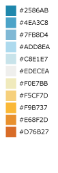
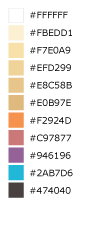
Blue to Orange
An 11-step diverging color ramp from blue to gray to orange. The gray critical class in the middle clearly shows a median or zero value. Example uses include temperature, climate, elevation, or other color ranges where it is necessary to distinguish categories with multiple hues.
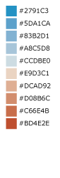
Blue to Red
A 10-step diverging color ramp from blue to red. Example uses include elections and politics, voter swing, climate or temperature, or other color ranges where it is necessary to distinguish categories with multiple hues.
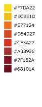
Green to Red-Orange
A 10-step diverging color ramp from green to red-orange. Example uses include elections and politics, voter swing, climate or temperature, or other color ranges where it is necessary to distinguish categories with multiple hues.
Green to Orange
A 13-step diverging color ramp from green to orange. Example uses include elevation, relief maps, topography, or other color ranges where it is necessary to distinguish categories with multiple hues.
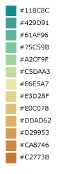
Light to Dark - Sunset
An 11-step sequential color ramp showing intensity from light to dark. This color ramp is perfect for showing density where it is critical to highlight very different values with bold colors at the higher, darker end of the ramp. Example uses include population density, accessibility, or ranking.
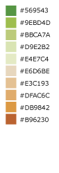
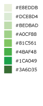
Light to Dark - Green
A basic 8-step sequential color ramp showing light to dark in shades of green. Example uses include density, ordered data, ranking, or any map where darker colors represent higher data values and lighter colors represent lower data values, generally.
Yellow to Red - Heatmap
An 8-step sequential heatmap from yellow to dark red. Great for heatmaps on a light basemap where the hottest values are more opaque or dark. Also useful for sequential color ranges where the lowest value is the median or zero value.
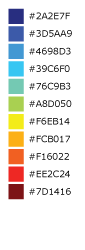
Blue to Yellow to Red Spectrum - Heatmap
An 11-step heatmap from blue to yellow to red. Great for showing a wide range of values with clear differences in hue.
Dark Red to Yellow-White - Heatmap
A 10-step sequential heatmap from dark red to yellow to white. Great for heatmaps where the hottest values should look more vibrant or intense.
Light Purple to Dark Purple to White
An 8-step sequential heatmap to show intensity with shades of purple with white as the “hottest” value. Great for light or gray basemaps, or where the highest value needs to be called out visually.
Bold Land Use
An 8-hue qualitative scheme used to show a clear difference in categories that are unordered or very different. Example uses include zoning, land use, land cover, or maps where all categories or groups are equal in visual strength/magnitude.
Muted Terrain
An 8-hue qualitative scheme used to show different kinds of map topology or features. This is generally used to show landforms, terrain, and topology.
Viridis, Magma, Plasma and Inferno
The Viridis, Magma, Plasma and Inferno color ramps were developed for matplotlib, and are incorporated into our default color ramp set. You can read more about these color ramps here <https://bids.github.io/colormap/>.
Custom Color Ramps
You can create your own color ramp with a list of integar values, constructed using our RBG or RGBA helper objects.
val colorRamp =
  ColorRamp(
    RGB(0,255,0),
    RGB(63, 255 ,51),
    RGB(102,255,102),
    RGB(178, 255,102),
    RGB(255,255,0),
    RGB(255,255,51),
    RGB(255,153, 51),
    RGB(255,128,0),
    RGB(255,51,51),
    RGB(255,0,0)
  )
You can also do things like set the number of stops in a gradient between colors, and set an alpha gradient. This example sets a 100 color stops that interpolates colors between red and blue, with an alpha value that starts at totally opaque for the red values, and ends at 0xAA alpha for blue values:
val colorRamp =
      ColorRamp(0xFF0000FF, 0x0000FFFF)
        .stops(100)
        .setAlphaGradient(0xFF, 0xAA)
There are many online and offline resources for generating color palettes for cartography including:
- Carto Colors
- ColorBrewer 2.0
- Cartographer’s Toolkit: Colors, Typography, Patterns, by Gretchen N. Peterson
- Designing Better Maps, by Cynthia A. Brewer
- Designed Maps: A Sourcebook, by Cynthia A. Brewer
RGBA vs RGB values
One way to represent a color is as an RGB hex value, as often seen in CSS or graphics programs. For example, the color red is represented by #FF0000 (or, in scala, 0xFF0000).
Internally to GeoTrellis, colors are represented as RGBA values, which includes a value for transparency. These can be represented with 8 instead of 6 hex characters (with the alpha opacity value being the last two charcters) such as 0xFF0000FF for opaque red. When using the programming interface, just be sure to keep the distinction in mind.
You can create RGB and RGBA colors in a variety of ways:
import geotrellis.raster.render._

val color1: Int = RGB(r = 255, g = 170, b = 85)
val color2: Int = RGBA(0xFF, 0xAA, 0x55, 0xFF)
val color3: Int = 0xFFAA55FF
assert(color1 == color2 && color2 == color3)
ColorMap
A ColorMap is what actually determines how the values of a tile to
colors. It constitutes a mapping between class break values and color
stops, as well as some options that determine how to color raster
values.
ColorMap Options
The options available for a ColorMap are a class boundary type, which
determines how those class break values (one of GreaterThan,
GreaterThanOrEqualTo, LessThan, LessThanOrEqualTo, or
Exact), an option that defines what color NoData values should be
colored, as well as an option for a “fallback” color, which determines
the color of any value that doesn’t fit to the color map. Also, if the
strict option is true, then no fallback color is used, and the code
will throw an exception if a value does not fit the color map. The
default values of these options are:
val colorMapDefaultOptions =
  ColorMap.Options(
    classBoundaryType = LessThan,
    noDataColor = 0x00000000, // transparent
    fallbackColor = 0x00000000, // transparent
    strict = false
  )
To examplify the options, let’s look at how two different color ramps will color values.
import geotrellis.render._

// Constructs a ColorMap with default options,
// and a set of mapped values to color stops.
val colorMap1 =
  ColorMap(
    Map(
      3.5 -> RGB(0,255,0),
      7.5 -> RGB(63,255,51),
      11.5 -> RGB(102,255,102),
      15.5 -> RGB(178,255,102),
      19.5 -> RGB(255,255,0),
      23.5 -> RGB(255,255,51),
      26.5 -> RGB(255,153,51),
      31.5 -> RGB(255,128,0),
      35.0 -> RGB(255,51,51),
      40.0 -> RGB(255,0,0)
    )
  )

// The same color map, but this time considering the class boundary type
// as GreaterThanOrEqualTo, and with a fallback and nodata color.
val colorMap2 =
  ColorMap(
    Map(
      3.5 -> RGB(0,255,0),
      7.5 -> RGB(63,255,51),
      11.5 -> RGB(102,255,102),
      15.5 -> RGB(178,255,102),
      19.5 -> RGB(255,255,0),
      23.5 -> RGB(255,255,51),
      26.5 -> RGB(255,153,51),
      31.5 -> RGB(255,128,0),
      35.0 -> RGB(255,51,51),
      40.0 -> RGB(255,0,0)
    ),
  ColorMap.Options(
    classBoundaryType = GreaterThanOrEqualTo,
    noDataColor = 0xFFFFFFFF,
    fallbackColor = 0xFFFFFFFF
  )
)
If we were to use the mapDouble method of the color maps to find
color values of the following points, we’d see the following:
scala> colorMap1.mapDouble(2.0) == RGB(0, 255, 0)
res1: Boolean = true

scala> colorMap2.mapDouble(2.0) == 0xFFFFFFFF
res2: Boolean = true
Because colorMap1 has the LessThan class boundary type, 2.0
will map to the color value of 3.5. However, because colorMap2
is based on the GreaterThanOrEqualTo class boundary type, and
2.0 is not greater than or equal to any of the mapped values, it
maps 2.0 to the fallbackColor.
scala> colorMap1.mapDouble(23.5) == RGB(255,153,51)
res4: Boolean = true

scala> colorMap2.mapDouble(23.5) == RGB(255,255,51)
res5: Boolean = true
If we map a value that is on a class border, we can see that the
LessThan color map maps the to the lowest class break value that our
value is still less than (26.5), and for the
GreaterThanOrEqualTo color map, since our value is equal to a class
break value, we return the color associated with that value.
Creating a ColorMap based on Histograms
One useful way to create ColorMaps is based on a Histogram of a
tile. Using a histogram, we can compute the quantile breaks that match
up to the color stops of a ColorRamp, and therefore paint a tile
based on quantiles instead of something like equal intervals. You can
use the fromQuantileBreaks method to create a ColorMap from both
a Histogram[Int] and Histogram[Double]
Here is an example of creating a ColorMap from a ColorRamp and a
Histogram[Int], in which we define a ramp from red to blue, set the
number of stops to 10, and convert it to a color map based on quantile
breaks:
val tile: Tile = ???

val colorMap = ColorMap.fromQuantileBreaks(tile.histogram, ColorRamp(0xFF0000FF, 0x0000FFFF).stops(10))
Here is another way to do the same thing, using the
ColorRamp.toColorMap:
val tile: Tile = ???

val colorMap: ColorMap =
  ColorRamp(0xFF0000FF, 0x0000FFFF)
    .stops(10)
    .toColorMap(tile.histogram)
PNG and JPG Settings
It might be useful to tweak the rendering of images for some use cases.
In light of this fact, both png and jpg expose a Settings classes
(geotrellis.raster.render.jpg.Settings and
geotrellis.raster.render.png.Settings) which provide a means to tune
image encoding.
In general, messing with this just isn’t necessary. If you’re unsure, there’s a good chance this featureset isn’t for you.
PNG Settings
png.Settings allows you to specify a ColorType (bit depth and
masks) and a Filter. These can both be read about on the W3
specification and png Wikipedia
page.
JPEG Settings
jpg.Settings allow specification of the compressionQuality (a Double
from 0 to 1.0) and whether or not Huffman tables are to be computed on
each run - often referred to as ‘optimized’ rendering. By default, a
compressionQuality of 0.7 is used and Huffman table optimization is not
used.
Resampling
Often, when working with raster data, it is useful to change the resolution, crop the data, transform the data to a different projection, or to do all of that at once. This all relies on our ability to resample, which is the act of changing the spatial resolution and layout of the raster cells, and interpolating the values of the modified cells from the original cells. For everything there is a price, however, and changing the resolution of a tile is no exception: there will (almost) always be a loss of information (or representativeness) when conducting an operation which changes the number of cells on a tile.
Upsampling vs Downsampling
Intuitively, there are two ways that you might resample a tile. You might:
- increase the number of cells
- decrease the number of cells
Increasing the number of cells produces more information at the cost of being only probabilistically representative of the underlying data whose points are being used to generate new values. We can call this upsampling (because we’re increasing the samples for a given representation of this or that state of affairs). Typically, upsampling is handled through interpolation of new values based on the old ones.
The opposite, downsampling, involves a loss of information. Fewer points of data are tasked with representing the same states of affair as the tile on which the downsampling is carried out. Downsampling is a common strategy in digital compression.
Aggregate vs Point-Based Resampling
In geotrellis, ResampleMethod is an ADT (through a sealed trait in
Resample.scala) which branches into PointResampleMethod and
AggregateResampleMethod. The aggregate methods of resampling are all
suited for downsampling only. For every extra cell created by upsampling
with an AggregateResampleMethod, the resulting tile is absolutely
certain to contain a NODATA cell. This is because for each
additional cell produced in an aggregated resampling of a tile, a
bounding box is generated which determines the output cell’s value on
the basis of an aggregate of the data captured within said bounding box.
The more cells produced through resampling, the smaller an aggregate
bounding box. The more cells produced through resampling, the less
likely it is that this box will capture any values to aggregate over.
What we call ‘point’ resampling doesn’t necessarily require a box within which data is aggregated. Rather, a point is specified for which a value is calculated on the basis of nearby value(s). Those nearby values may or may not be weighted by their distance from the point in question. These methods are suitable for both upsampling and downsampling.
Remember What Your Data Represents
Along with the formal characteristics of these methods, it is important
to keep in mind the specific character of the data that you’re working
with. After all, it doesn’t make sense to use a method like Bilinear
resampling if you’re dealing primarily with categorical data. In this
instance, your best bet is to choose an aggregate method (and keep in
mind that the values generated don’t necessarily mean the same thing as
the data being operated on) or a forgiving (though unsophisticated)
method like NearestNeighbor.
Histograms
It’s often useful to derive a histogram from rasters, which represents a
distribution of the values of the raster in a more compact form. In
GeoTrellis, we differentiate between a Histogram[Int], which represents
the exact counts of integer values, and a Histogram[Double], which
represents a grouping of values into a discrete number of buckets. These
types are in the geotrellis.raster.histogram package.
The default implementation of Histogram[Int] is the
FastMapHistogram, developed by Erik Osheim, which utilizes a growable
array structure for keeping track of the values and counts.
The default implementation of Histogram[Double] is the
StreamingHistogram, developed by James McClain and based on the paper
Ben-Haim, Yael, and Elad Tom-Tov. "A streaming parallel decision tree
algorithm."  The Journal of Machine Learning Research 11 (2010): 849-872.
.
Histograms can give statistics such as min, max, median, mode and median. It also can derive quantile breaks, as dsecribed in the next section.
Quantile Breaks
Dividing a histogram distribution into quantile breaks attempts to classify values into some number of buckets, where the number of values classified into each bucket are generally equal. This can be useful in representing the distribution of the values of a raster.
For instance, say we had a tile with mostly values between 1 and 100, but there were a few values that were 255. We want to color the raster with 3 values: low values with red, middle values with green, and high values with blue. In other words, we want to classify each of the raster values into one of three categories: red, green and blue. One technique, called equal interval classification, consists of splitting up the range of values (1 - 255) into the number of equal intervals as target classifications (3). This would give us a range intervals of 1 - 85 for red, 86 - 170 for green, and 171 - 255 for blue. This corresponds to “breaks” values of 85, 170, and 255. Because the values are mostly between 1 and 100, most of our raster would be colored red. This may not show the contrast of the dataset that we would like.
Another technique for doing this is called quantile break classification; this makes use of the quantile breaks we can derive from our histogram. The quantile breaks will concentrate on making the number of values per “bin” equal, instead of the range of the interval. With this method, we might end up seeing breaks more like 15, 75, 255, depending on the distribution of the values.
For a code example, this is how we would do exactly what we talked about: color a raster tile into red, green and blue values based on it’s quantile breaks:
import geotrellis.raster.histogram._
import geotrellis.raster.render._

val tile: Tile = ???  // Some raster tile
val histogram: Histogram[Int] = tile.histogram

val colorRamp: ColorRamp =
  ColorRamp(
    RGB(r=0xFF, b=0x00, g=0x00),
    RGB(r=0x00, b=0xFF, g=0x00),
    RGB(r=0x00, b=0x00, g=0xFF)
  )

val colorMap = ColorMap.fromQuantileBreaks(histogram, colorRamp)

val coloredTile: Tile = tile.color(colorMap)
Kriging Interpolation
These docs are about Raster Kriging interpolation.
The process of Kriging interpolation for point interpolation is explained in the geotrellis.vector.interpolation package documnetation.
Kriging Methods
The Kriging methods are largely classified into different types in the way the mean(mu) and the covariance values of the object are dealt with.
// Array of sample points with given data
val points: Array[PointFeature[Double]] = ...
/** Supported is also present for
  * val points: Traversable[PointFeature[D]] = ... //where D <% Double
  */

// The raster extent to be kriged
val extent = Extent(xMin, yMin, xMax, yMax)
val cols: Int = ...
val rows: Int = ...
val rasterExtent = RasterExtent(extent, cols, rows)
There exist four major kinds of Kriging interpolation techniques, namely:
Simple Kriging
// Simple kriging, a tile  set with the Kriging prediction per cell is returned
val sv: Semivariogram = NonLinearSemivariogram(points, 30000, 0, Spherical)

val krigingVal: Tile = points.simpleKriging(rasterExtent, 5000, sv)

/**
  * The user can also do Simple Kriging using :
  * points.simpleKriging(rasterExtent)
  * points.simpleKriging(rasterExtent, bandwidth)
  * points.simpleKriging(rasterExtent, Semivariogram)
  * points.simpleKriging(rasterExtent, bandwidth, Semivariogram)
  */
It belong to the class of Simple Spatial Prediction Models.
The simple kriging is based on the assumption that the underlying stochastic process is entirely known and the spatial trend is constant, viz. the mean and covariance values of the entire interpolation set is constant (using solely the sample points)
mu(s) = mu              known; s belongs to R
cov[eps(s), eps(s')]    known; s, s' belongs to R
Ordinary Kriging
// Ordinary kriging, a tile  set with the Kriging prediction per cell is returned
val sv: Semivariogram = NonLinearSemivariogram(points, 30000, 0, Spherical)

val krigingVal: Tile = points.ordinaryKriging(rasterExtent, 5000, sv)

/**
  * The user can also do Ordinary Kriging using :
  * points.ordinaryKriging(rasterExtent)
  * points.ordinaryKriging(rasterExtent, bandwidth)
  * points.ordinaryKriging(rasterExtent, Semivariogram)
  * points.ordinaryKriging(rasterExtent, bandwidth, Semivariogram)
  */
It belong to the class of Simple Spatial Prediction Models.
This method differs from the Simple Kriging appraoch in that, the constant mean is assumed to be unknown and is estimated within the model.
mu(s) = mu              unknown; s belongs to R
cov[eps(s), eps(s')]    known; s, s' belongs to R
Universal Kriging
// Universal kriging, a tile  set with the Kriging prediction per cell is returned
val attrFunc: (Double, Double) => Array[Double] = {
  (x, y) => Array(x, y, x * x, x * y, y * y)
}

val krigingVal: Tile = points.universalKriging(rasterExtent, attrFunc, 50, Spherical)

/**
  * The user can also do Universal Kriging using :
  * points.universalKriging(rasterExtent)
  * points.universalKriging(rasterExtent, bandwidth)
  * points.universalKriging(rasterExtent, model)
  * points.universalKriging(rasterExtent, bandwidth, model)
  * points.universalKriging(rasterExtent, attrFunc)
  * points.universalKriging(rasterExtent, attrFunc, bandwidth)
  * points.universalKriging(rasterExtent, attrFunc, model)
  * points.universalKriging(rasterExtent, attrFunc, bandwidth, model)
  */
It belongs to the class of General Spatial Prediction Models.
This model allows for explicit variation in the trend function (mean function) constructed as a linear function of spatial attributes; with the covariance values assumed to be known. This model computes the prediction using
For example if:
x(s) = [1, s1, s2, s1 * s1, s2 * s2, s1 * s2]'
mu(s) = beta0 + beta1*s1 + beta2*s2 + beta3*s1*s1 + beta4*s2*s2 + beta5*s1*s2
Here, the “linear” refers to the linearity in parameters (beta).
mu(s) = x(s)' * beta,   beta unknown; s belongs to R
cov[eps(s), eps(s')]    known; s, s' belongs to R
Geostatistical Kriging
// Geostatistical kriging, a tile  set with the Kriging prediction per cell is returned
val attrFunc: (Double, Double) => Array[Double] = {
  (x, y) => Array(x, y, x * x, x * y, y * y)
}

val krigingVal: Tile = points.geoKriging(rasterExtent, attrFunc, 50, Spherical)

/**
  * The user can also do Universal Kriging using :
  * points.geoKriging(rasterExtent)
  * points.geoKriging(rasterExtent, bandwidth)
  * points.geoKriging(rasterExtent, model)
  * points.geoKriging(rasterExtent, bandwidth, model)
  * points.geoKriging(rasterExtent, attrFunc)
  * points.geoKriging(rasterExtent, attrFunc, bandwidth)
  * points.geoKriging(rasterExtent, attrFunc, model)
  * points.geoKriging(rasterExtent, attrFunc, bandwidth, model)
  */
It belong to the class of General Spatial Prediction Models.
This model relaxes the assumption that the covariance is known. Thus, the beta values and covariances are simultaneously evaluated and is computationally more intensive.
mu(s) = x(s)' * beta,   beta unknown; s belongs to R
cov[eps(s), eps(s')]    unknown; s, s' belongs to R
Attribute Functions (Universal, Geostatistical Kriging):
The attrFunc function is the attribute function, which is used for
evaluating non-constant spatial trend structures. Unlike the Simple and
Ordinary Kriging models which rely only on the residual values for
evaluating the spatial structures, the General Spatial Models may be
modelled by the user based on the data (viz. evaluating the beta
variable to be used for interpolation).
In case the user does not specify an attribute function, by default the
function used is a quadratic trend function for Point(s1, s2) :
mu(s) = beta0 + beta1*s1 + beta2*s2 + beta3*s1*s1 + beta4*s2*s2 + beta5*s1*s2
General example of a trend function is :
mu(s) = beta0 + Sigma[ beta_j * (s1^n_j) * (s2^m_j) ]
Example to understand the attribute Functions
Consider a problem statement of interpolating the ground water levels of Venice. It is easy to arrive at the conclusion that it depends on three major factors; namely, the elevation from the ground, the industries’ water intake, the island’s water consumption. First of all, we would like to map the coordinate system into another coordinate system such that generation of the relevant attributes becomes easier (please note that the user may use any method for generating the set of attribute functions; in this case we have used coordinate transformation before the actual calculation).
val c1: Double = 0.01 * (0.873 * (x - 418) - 0.488 * (y - 458))
val c2: Double = 0.01 * (0.488 * (x - 418) + 0.873 * (y - 458))
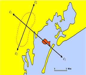
Coordinate Mapping
Image taken from
Smith, T.E., (2014) Notebook on Spatial Data Analysis [online] http://www.seas.upenn.edu/~ese502/#notebook
Elevation
/** Estimate of the elevation's contribution to groundwater level
  * [10 * exp(-c1)]
  */
val elevation: Double = math.exp(-1 * c1)
Industry draw down (water usage of industry)
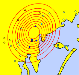
Industry Draw Down
Image taken from
Smith, T.E., (2014) Notebook on Spatial Data Analysis [online] http://www.seas.upenn.edu/~ese502/#notebook
/** Estimate of the industries' contribution to groundwater level
  * exp{ -1.0 * [(1.5)*c1^2 - c2^2]}
  */
val industryDrawDown: Double = math.exp(-1.5 * c1 * c1 - c2 * c2)
Island draw down (water usage of Venice)
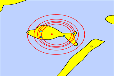
Venice Draw Down
Image taken from
Smith, T.E., (2014) Notebook on Spatial Data Analysis [online] http://www.seas.upenn.edu/~ese502/#notebook
/** Estimate of the island's contribution to groundwater level
  * //exp{-1.0 * (sqrt((s1-560)^2 + (s2-390)^2) / 35)^8 }
  */
val islandDrawDown: Double =
    math.exp(-1 * math.pow(math.sqrt(math.pow(x - 560, 2) + math.pow(y - 390, 2)) / 35, 8))
The Final Attribute Function
Thus for a Point(s1, s2) :
Array(elevation, industryDrawDown, islandDrawDown) is the set of
attributes.
In case the intuition for a relevant attrFunc is not clear; the user
need not supply an attrFunc, by default the following attribute
Function is used :
// For a Point(x, y), the set of default attributes is :
Array(x, y, x * x, x * y, y * y)
The default function would use the data values of the given sample points and construct a spatial structure trying to mirror the actual attribute characteristics.